
Hello all and welcome back to the Excel Tip of the Week! This week, we have a Basic User post in which we are refreshing our coverage of the quintessential data navigation feature, the filter.
Filters can be used to sort or hide items from a block of data. By default, you can switch them on simply by pressing the Data => Filter button while any cell in the data is active:
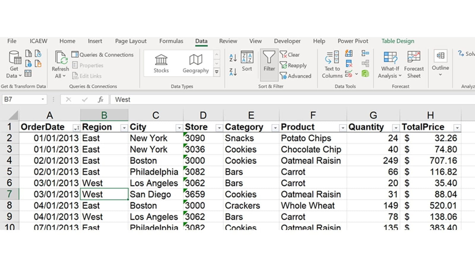
How to apply filters
These also come automatically if you make your data into an Excel Table with Ctrl T or from the Home menu – which I thoroughly recommend for reasons I won’t expand on here.
Note that this automatic labelling isn’t perfect – it will go out in each direction until it finds blank rows and blank columns to serve as the borders of your data. If your data has gaps in it, you can overrule this by first selecting all the data you want to filter, then hitting the button.
What filters can do for you
Filters work using the small down-arrow “handles” shown at the top of each column. These open up a menu which lets you easily work with the data in that column. Any changes you make – such as sorting that column into a different order, or using the values in that column to filter out some rows – will be applied across the entire dataset. Note that filtering hides the entire row, so anything that’s adjacent to the data will also be hidden. For this reason, best practice is not to put other things alongside filtered data.
The exact menu you get is context-dependent based on what kind of data Excel detects is in the column. There are three versions for numeric data, date-and-time data, and text data. We’ll examine each in turn.
Numeric data
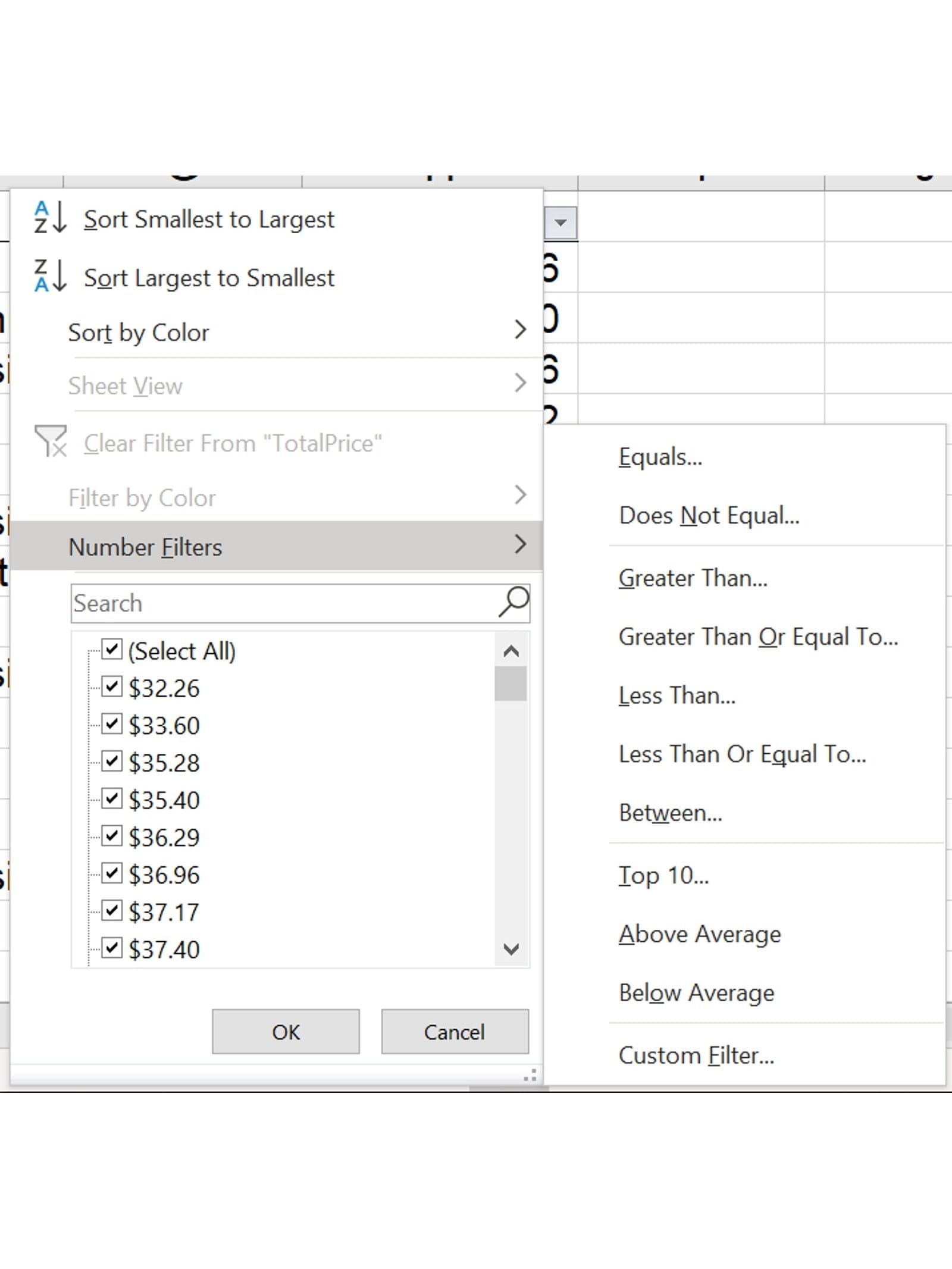
Here the sort options are in size order. You can use the checkboxes to manually hide & unhide certain items. The expanded “Number filters” menu has various standard numeric searches available, plus an option to design your own, such as a “not between” filter which is useful for finding material amounts in a mixed column of positive and negative numbers.
Date-and-time data
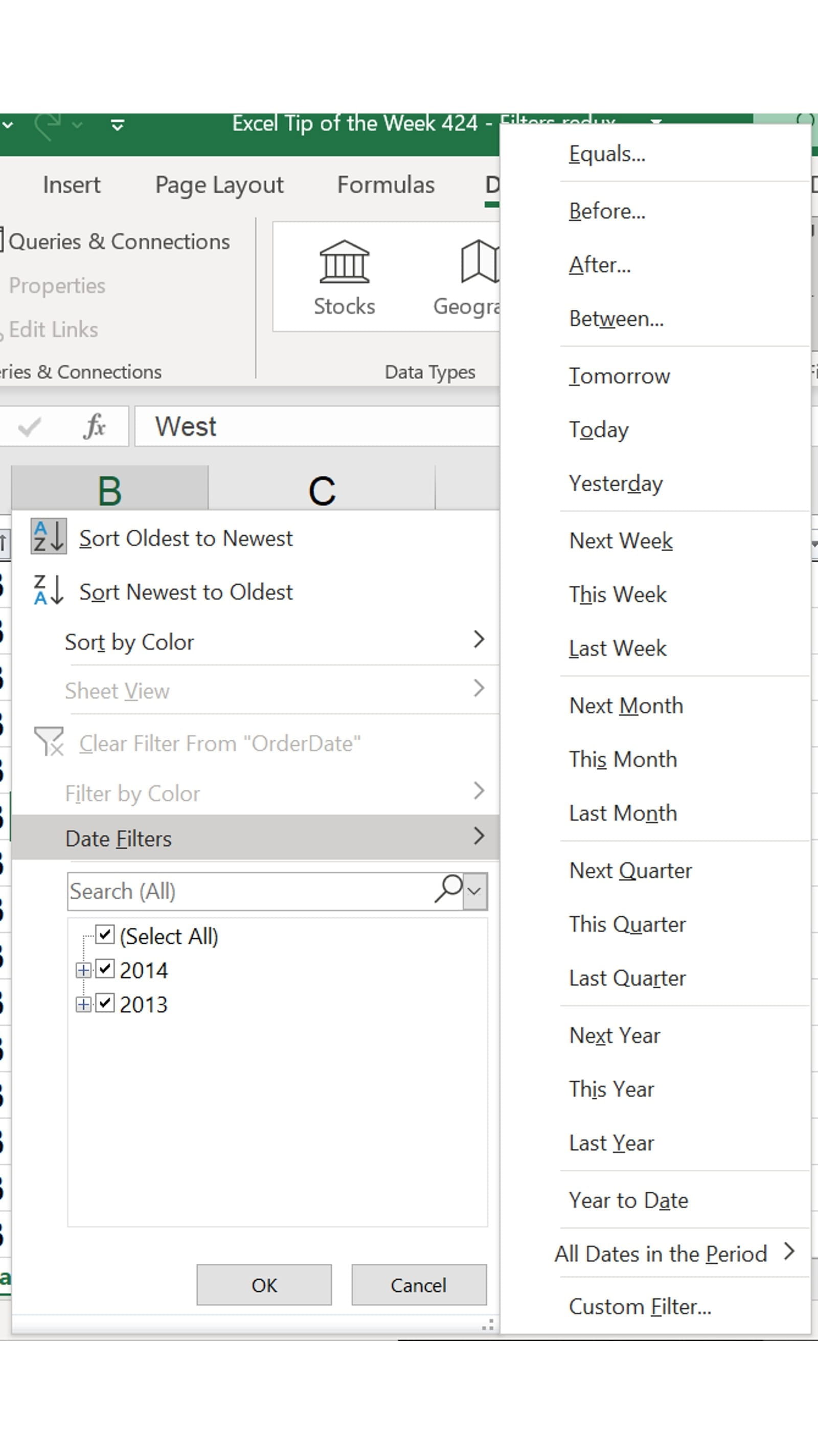
Now the sort options are for chronological order. The default behaviour for the tickboxes is to group any dates into collapsible year-month-day tiers, which you can see here (the ‘+’ will expand to show the next level down). The expandable date filters include a wide variety of time-based filters. Annoyingly, these don’t include “before today” or “after today”, which you would have to do with an additional formula column or a VBA filter.
Text data
Anything that Excel can’t parse as either of the above two gets the text data menu:
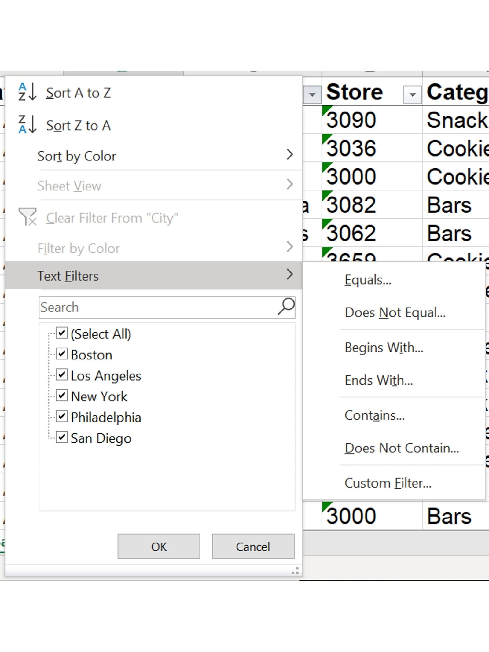
The sort options are for alphabetical sorting, unsurprisingly. There are a small number of expandable text filters also.
Working with filters
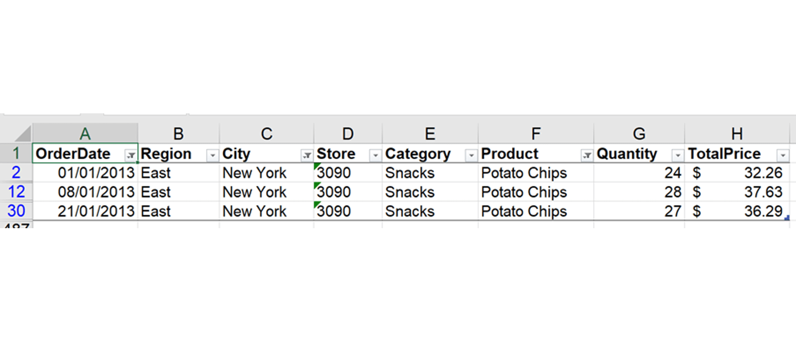
Each filter works on just one column (see TOTW #287 on Advanced Filter if you want to work with conditions that consider multiple columns). However you can cumulatively create a more complex filter by filtering columns one at a time. For example, you could find the potato chips ordered by the New York store in January 2013 by applying each filter consecutively:
Once you’ve done that, you might want to update or edit the data you find; if you do, you might notice that changing a row so it now falls outside of a filter won’t immediately make that row disappear – so if for example you corrected the item on row 12 to be for the San Diego store instead, it would still remain visible. Once you are done making changes, you can use Data => Reapply or Ctrl Alt L to refresh the filtering and make the row disappear. That same menu also has a Clear button if you want to remove all three column filters at once.
Another neat feature of filters is the ability to sort or filter by cell fill colour or font colour. This can be used to quickly find items that have been labelled, either manually or with conditional formatting. You can also use it to shorthand more complex filters like the above example – so you could find your particular target items, colour the rows in green, and then later on find them again with just a single fill colour filter rather than redoing all three column filters.
An important thing to remember is that Excel can only sort with the three types mentioned above. If your data is sorted in some other way, and you want to sort it temporarily to check something and then put it back, you’d better to remember to add a row number column first – or your custom sort will be lost forever!
You can experiment with all the various filtering options using this week’s example file.
- Excel Tips & Tricks #489 – The basics of charts in Excel part 2: Combo charts
- Excel Tips & Tricks #488 – The basics of charts in Excel
- Excel Tips & Tricks #487 – An Introduction to Slicers
- Excel Tips & Tricks #486 – Revisiting inserting hyperlinks
- Excel Tips & Tricks #485 – Refreshing NETWORKDAYS and WORKDAY functions
Archive and Knowledge Base
This archive of Excel Community content from the ION platform will allow you to read the content of the articles but the functionality on the pages is limited. The ION search box, tags and navigation buttons on the archived pages will not work. Pages will load more slowly than a live website. You may be able to follow links to other articles but if this does not work, please return to the archive search. You can also search our Knowledge Base for access to all articles, new and archived, organised by topic.
