Mastering number formats - part 2

This is the second part of our new series and the second part of a guide to Excel number formats. Having covered basic custom formats last time, this time we are going to explore some slightly more complicated aspects of number formats, including how best to make them easily accessible in your spreadsheets.

Below is the example we used in part 1, except for a change to one of the two values that were previously set at 0. We have changed one of these to £400. As you can see, despite setting our number format to show 0 as a dash, one of our formatted 0s is showing as 0 rather than -. This is because the underlying value isn't zero, it's 400 that is then rounded down to 0. We are going to start this article by looking at a format that shows values in £'000 before trying to deal with non-zero values that are rounded to 0:

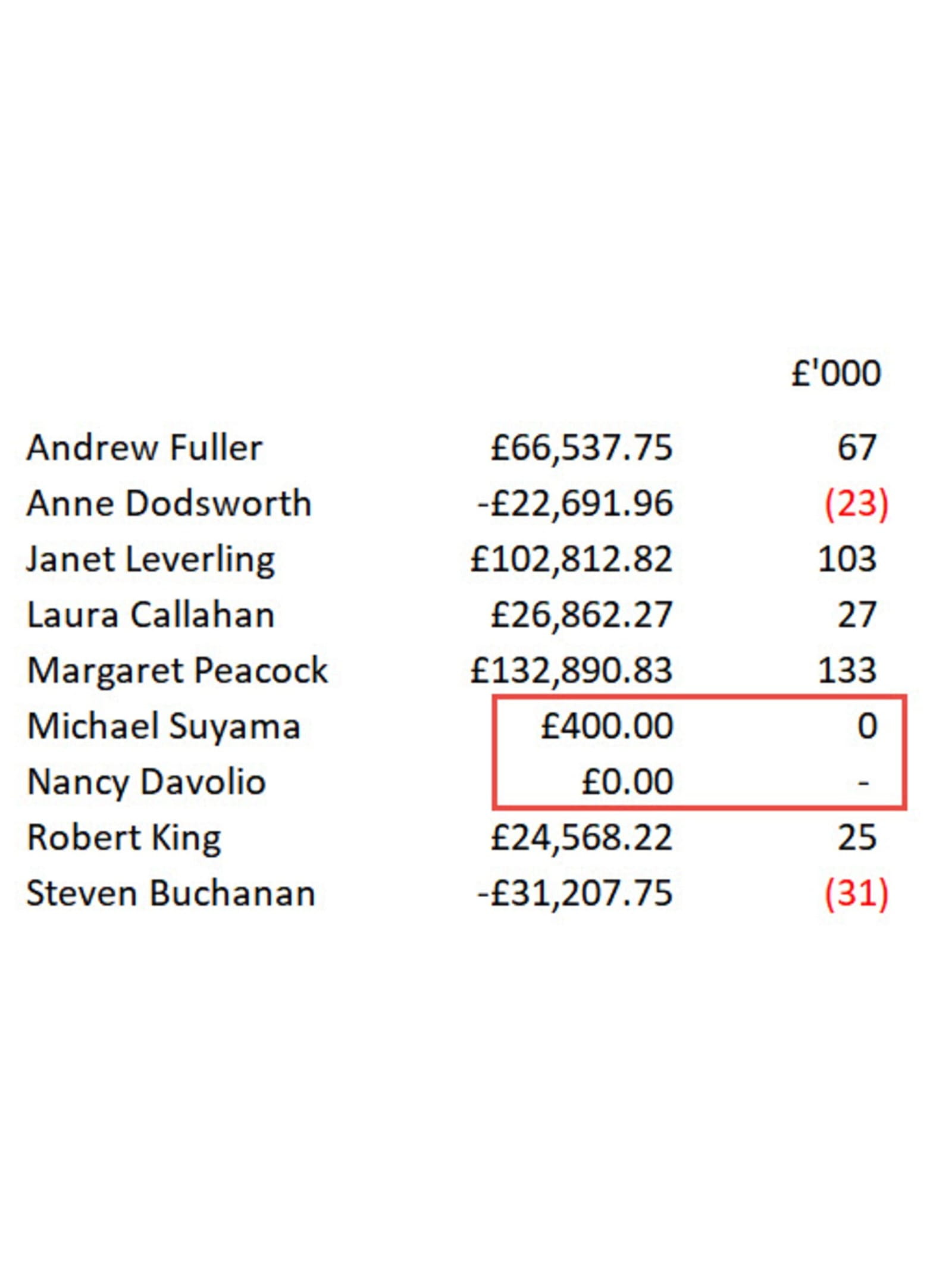
Here is the custom format we are using in our £'000 column:

#,##0,_);[Red](#,##0,);-?

As well as the comma that sets the thousand separators between the digits 3^rd and 4^th from the right, there is an additional comma to the right of each of the rightmost digits in each section. It is this comma that causes the display of our numbers to be in thousands. Each additional comma after the rightmost digit 'rounds' the display by a further 3 digits, so:

#,##0,,_);

would display to millions.

There are different ways to deal with the value rounded to zero issue. We could use the ROUND(() function to round our formatted value to thousands:

=ROUND(H8,-3)

Because our value would now really be zero rather than 400, the zero section of our custom number format would be applied and our cell would display a dash rather than 0. However, rounding obviously reduces the precision of the values so isn't always appropriate where we need to use the values in subsequent calculations. It is (almost) possible to solve the problem just using a custom format.

Although we generally think of the first two sections of our custom number format as being used to format all positive and all negative numbers respectively, we can define exactly which values these formats are applied to using comparison operators. Here we are limiting our first section to numbers above 500 and our negative section to numbers below -500:

[>=500]#,##0,_);[Red][<-500](#,##0,);-_)

This comes close to what we want to achieve but there is a strange issue. Values between the two criteria are formatted using the third section but -? displays, for example, -499 rather than the expected dash followed by a space character. Using dash followed by _) gives us a dash for a positive number below 500 followed by a space as wide as a closing bracket. However, for a negative number up to -499, the negative minus is still displayed by section 3, giving us --. So, if you like a challenge, see if you can come up with a custom format that gives a single dash for both positive and negative zeros.

Only the first two sections of a custom number format can use a condition, and the condition is entered in the form of a comparison operator (<> = etc.) and a number, all within a set of square brackets. If you are using conditions within a custom number format, the third section of the format will be used for any number that doesn't match a condition. If a condition is not specified in one of the first two sections, the default condition of positive for the first section and negative for the second section will apply. Note that the conditions are evaluated from left to right, so:

[Red][>100]#,##0;[Blue][>500]#,##0;[Green]#,##0

would show all numbers above 100, including those above 500, in red.

Using the format

Having come up with our perfect custom number format we will probably want to make it as easy to use as possible. Just creating a custom number format in a workbook only makes it available in the list of custom number formats for that workbook.

To make it easier to get at the format you could create a macro by recording the application of your new custom format, and then include a button to run the macro in a convenient place on the toolbar.

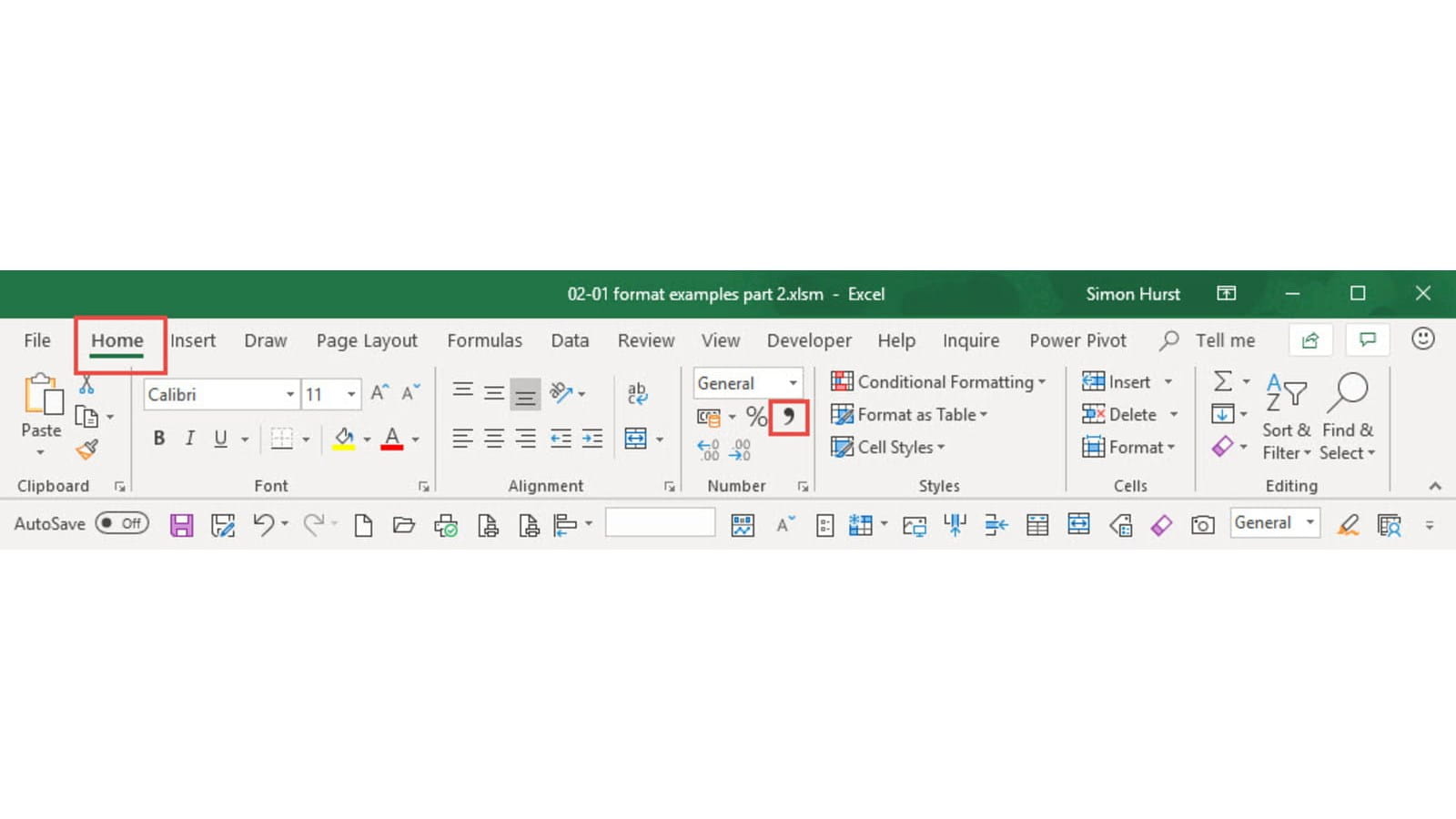
If you wish to avoid macros and Visual Basic for Applications code, then you can use an Excel cell style instead. Rather than needing to go to the Format Cells dialog, Number tab, to choose the new custom format which should be at the bottom of the list, we can easily attach our format to a Ribbon Tab button allowing it to be applied with a single click. The Number group of the Home Ribbon Tab includes a set of three buttons that apply Excel number styles: Currency, Percent and Comma. The obvious one to use is the Comma style. We just need to right-click on the Comma style in the Number Format section of the Excel Cell Styles gallery and choose Modify. We can then click on the Format button to choose our custom number format:

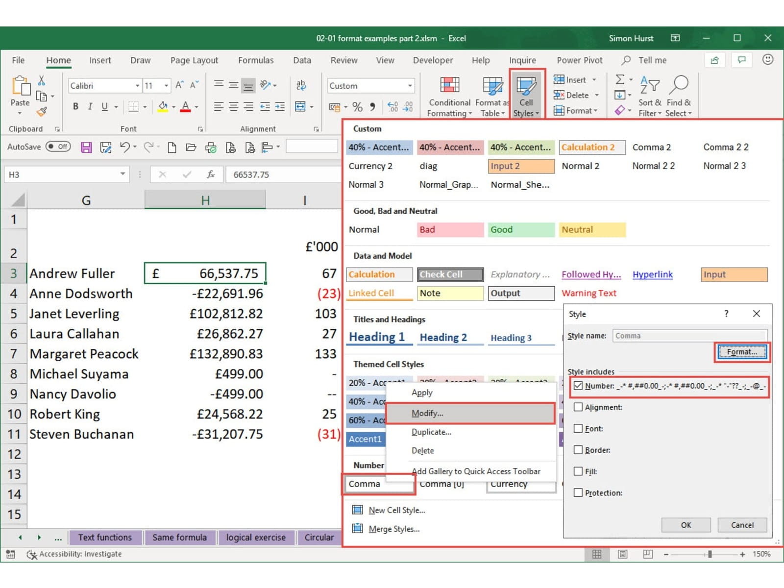
Once we have changed the number format of the Comma style, clicking on the Comma style button in the Number group will apply our custom format:

Unlike Word styles, which can automatically be added to the underlying template file, in Excel, cell styles just belong to the current workbook. The Merge Styles… command at the bottom of the Cell Styles gallery allows you to import styles from another open Excel workbook.

To make the new style generally available, you can modify the comma style in a workbook called Book.xltx in your XLSTART folder. You can go to File, Options, Trust Centre, Trust Centre Settings…, Trusted Locations to find the XLSTART folder location on your system. This workbook is used as the default for all new workbooks. If you find an existing book.xltx workbook then you could open it and merge your new comma style into it. If book.xltx doesn’t exist, then you will need to create it. Perhaps the easiest way is to start with a new blank workbook and merge your style into that new workbook. You can then use File, Save As to save that new workbook as an Excel Template by choosing that option from the Save As Type box. You will then need to navigate to the XLSTART folder location described above.

When a template named book.xltx exists in Excel’s XLSTART folder it will be used as the ‘template’ for creating a new workbook using the Control+N keyboard shortcut or the New button in the Quick Access Toolbar. Similarly, sheet.xltx will be the default for a new sheet inserted into a workbook.