
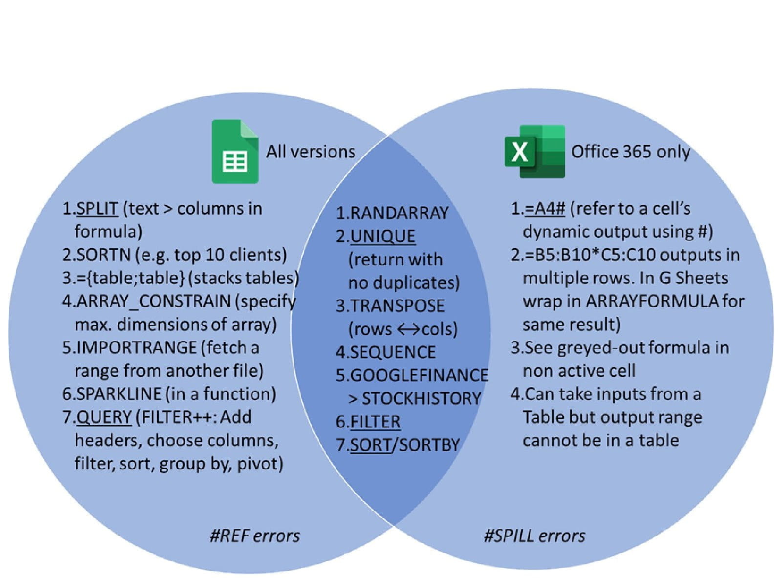
Excel heralded dynamic arrays as a revolutionary change. I don’t disagree, developers rebuilt Excel’s formula engine from the ground up to allow for them, but Google Sheets has had dynamic arrays for a while, (although it had never been given that name). They diverge though, standout differences are in Excel you can refer to the dynamic spill range using the # character whereas Google Sheets can stack two tables together, has SPLIT, SORTN, and the flexible QUERY function, a super powered FILTER where you choose columns and see headers. This Venn diagram summarises the similarities & differences.
What are dynamic arrays?
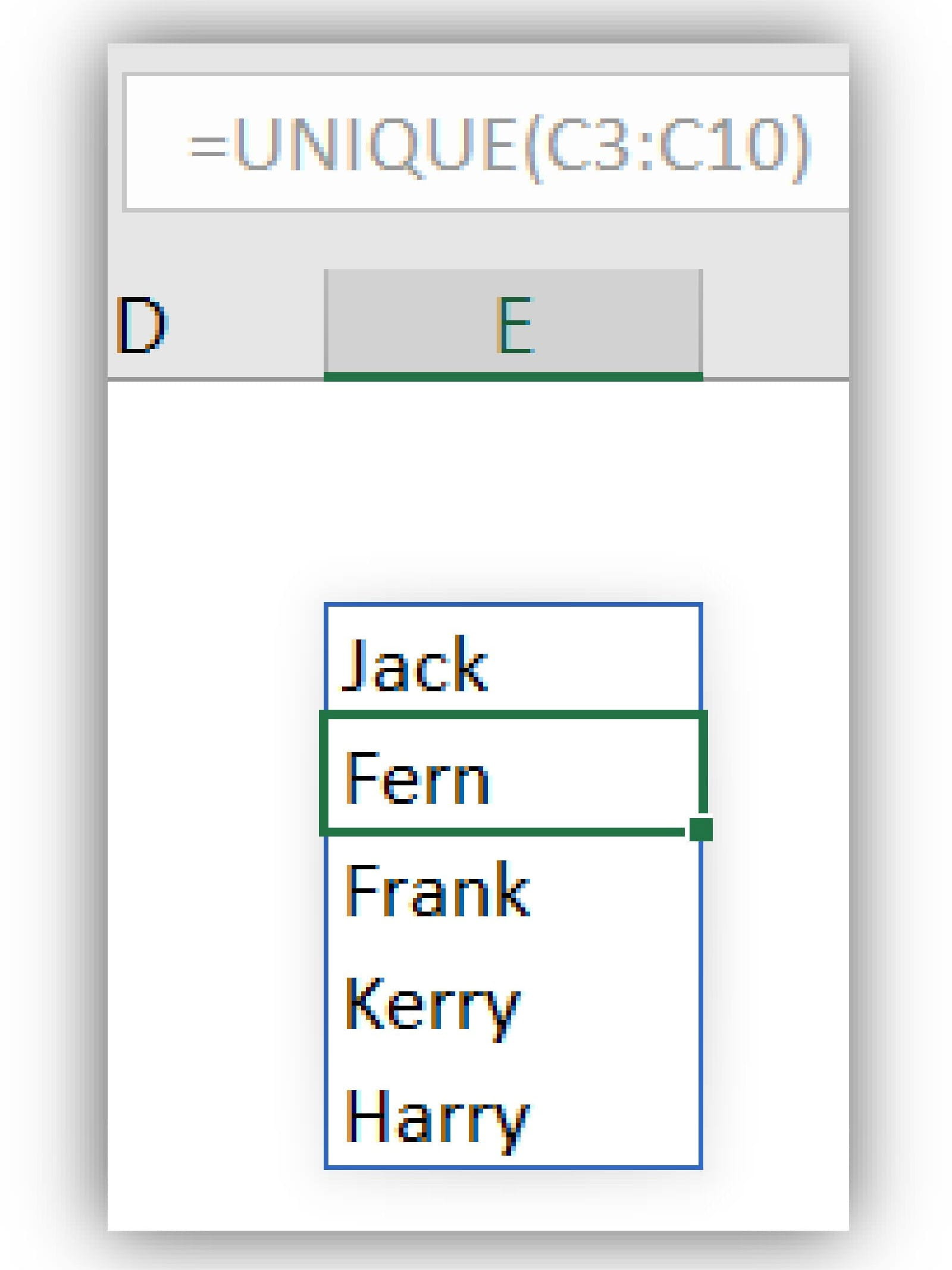
At its core, dynamic arrays, is the ability for a formula to return a table (with multiple columns & rows) rather than a single value. Let’s look at my favourite: The UNIQUE function returns a unique list of text values based on another list which may contain duplicates using =UNIQUE(list), you can also wrap it in a SORT function to sort the output from A to Z by writing =SORT(UNIQUE(list)). Both Excel and Google Sheets does this the same way.
Multiple Google Sheets dynamic arrays functions & methods are covered in this video:
Excel Dynamic arrays’ best and worst five features are covered in this video:
The user interface (Winner Excel)
Excel will wrap the SPILL range (i.e. the table output) within a blue box and when you click on an output cell (i.e. where the output exists but that is not the root cell), you will see the formula greyed out (so it can be viewed but not edited). Google doesn’t provide any of these user interface benefits, and if you click on a non-root cell, it just shows the output value.
Compatibility (Winner Sheets)
Excel’s dynamic Arrays only work within Excel with Microsoft 365 whereas Google Sheets’ main overarching advantage over Excel is that everyone has the same version on every device, there’s no concept of 2010 version vs 2016 or 365 version as its always the same. Yes, Excel Online does have dynamic arrays but personally I find Excel Online is lacking too many features to be usable.
Error handling (Winner Excel)
Excel shows its errors as #SPILL, whereas Google Sheets shows it as #REF errors. In both cases if you hover it will explain the errors (which in most cases is the obstructing cell), but Excel provides more explanation.
Formatting (Winner Sheets)
Google Sheets takes the number formatting (dates, percentage etc.) from the source data whereas Excel takes the formats of the output range, cell by cell (i.e. the formatting is not influenced by the dynamic array formulas).
Excel’s Table feature is an unsung hero by most who don’t know it however it is incompatible with dynamic arrays, outputs will give an error if they are in a Table (whereas input cells can be from a table). Google Sheets doesn’t have a Table feature, but it has a halfway alternative called “Alternating colours” under the format tab which does support dynamic arrays.
Functions available in both (Winner Sheets)
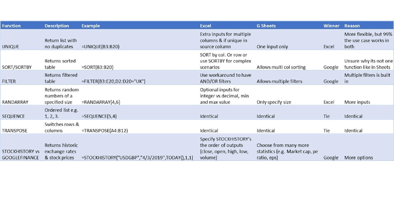
UNIQUE, SORT, FILTER, SEQUENCE, TRANSPOSE, RANDARRAY work in both applications, with slight differences, then Excel has SORTBY to make up for limitations in its version of SORT (whereas Google can do these features in SORT) and for getting historic stock/exchange prices there’s GOOGLEFINANCE or STOCKHISTORY in Excel. This table compares the two. I understand that there are workarounds to reproduce what one does in the other but for this article I will look at the core functionality without workarounds.
Google finance can be explored in more detail in this video:
FILTER and SORT are fantastic functions with two huge limitations:
- You must return the columns in the pre-specified order
- Headers need to manually be written on top of the formula in separate cells which to me feels like it loses the dynamic nature of it.
Fortunately, Google sheets has an answer…
QUERY (only in Sheets)
QUERY is by far the most sophisticated and flexible function in both Excel and Google Sheets. Although it gets complex, its base use case is incredibly useful (overcoming FILTER’s two limitations). =QUERY(source data,query,[headers]), the source data is like any dynamic array, the header input I usually leave blank (then it returns your headers) and the query part is the challenge, this allows you to write SQL like code in the formula, but don’t let that intimidate you – learn these simple things to start.
- Start with SELECT
- Write the requested column letters separated with commas, B, D, A (in any order)
- Type WHERE
- Type the column letter the = then the criteria which is wrapped in single quotes
- Wrap the entire query in double quotes
As explained QUERY gets more complicated, for me, filtering with WHERE is what I use 90% of the time but you can also filter for contains, starts with, dates, not plus you can order by, rename columns, specify output number formats and even replicate pivot tables with group by and pivot. Here is a complete guide to QUERY:
Stack different tables (only in Google Sheets)
One of my favourites is the ability to append two tables on top of each other. ={Cell range 1 with headers;Cell range 2 no headers} will do this e.g. ={A4:D8;A13:D16}.
To make the range dynamic, it’s a little togher as Google sheets doesn’t have the table feature so I recommend nesting a larger area inside a FILTER or QUERY function which then filters out blanks, so use either =FILTER({A4:D10;A13:D21},{A4:A10;A13:A21}<>"") or QUERY({A4:D10;A13:D19},"select * where Col1 is not null"). As I explained QUERY gets complex and uses different language.
SPLIT (Only in Sheets)
Split text to columns through a dynamic formula, useful for first/last names or hierarchal data. =SPLIT(cell ref, delimiter), You can specify one or multiple characters as a delimiter (wrapped in speech marks), but it will look for each character separately, not the combination of many characters (or criteria). E.g. SPLIT(A4,">-"), the last two optional inputs are rarely worthwhile.
ARRAY_CONSTRAIN (Sheets only)
Sometimes you want to ensure that an ARRAY doesn’t expand past a certain point, e.g. a maximum of 4 rows and 8 columns. =ARRAY_CONSTRAIN(Output of Array formula, max rows, max columns) so =ARRAY_CONSTRAIN(FILTER(A5:D200, A5:A200=”France”, 20,5) will limit the outputs to the first 20 rows it finds so you can safely use rows below.
SORTN (Sheets only)
ARRAY_CONSTRAIN limits the top rows but often you would want to limit by a sort column of choice. Other use cases are answering questions like “who were the top 5 customers or the bottom 10 salespeople. Additionally, you can wrap it in a SUM to get the sum of the top 5 sales. You can sort by one or multiple columns like in the SORT function. =SORTN(Range,[n],[display ties mode],[sort col],[is asc],[sort col 2]…) An example is =SORTN(B5:E15,5,,E5:E15,false) will give the rows filtered & sorted for the top 5 sorted by column E, whereas =SORTN(E5:E15,5) will output the bottom 5 rows in that range and can be nested inside a SUM. Text, numbers and dates can be sorted. I personally find it counter intuitive that the default sort order is bottom to top (equivalent to writing TRUE), but as always in Google Sheets, there’s always the QUERY function to rewrite it.
IMPORTRANGE (Sheets only)
In Excel, you can easily link two workbooks together by typing = and clicking on a cell in another workbook. In Google, the process is a little trickier to set it, but its more robust so personally, I prefer it. =IMPORTRANGE(spreadsheet URL, range) requires you to copy the URL from the source file, paste the into the first input (wrapped in double quotations), then type the range also in double quotations “sheet!Range”.
For example: =IMPORTRANGE("https://docs.google.com/spreadsheets/d/.../edit#gid=15234231634","Sales Sheet!A3:C10"). You may get an error but click on the error then “allow access” should fix it. Make sure you enter the punctuation correctly as debugging it can be tricky.

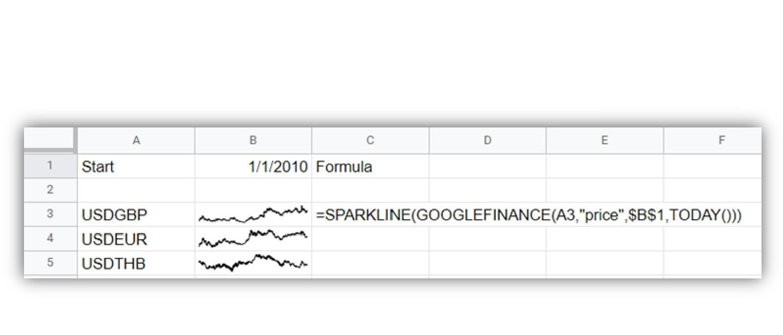
SPARKLINE (Winner Sheets)
Excel’s SPARKLINE is a command on the Insert tab, but Sheets equivalent is a function. In its simplest (and most common) form SPARKLINE creates a line chart in a cell and can have a dynamic array nested inside. If you explore the options, you can replicate many of Excel’s sparkline options or data bars (which Excel classifies under conditional formatting).
Making any formula a dynamic array (Winner Excel)
Dynamic arrays are much more than just new functions, any formula can now return multiple rows and columns, so for example =A3:A15*B3:B15 will return 13 values, rather than just one.

In Google Sheets, this experience is possible but with an additional step, =A3:A15*B3:B15 will return one value but if you nest it inside a function called ARRAYFORMULA, it will return 13 just like Excel. =ARRAYFORMULA(A3:A15*B3:B15)
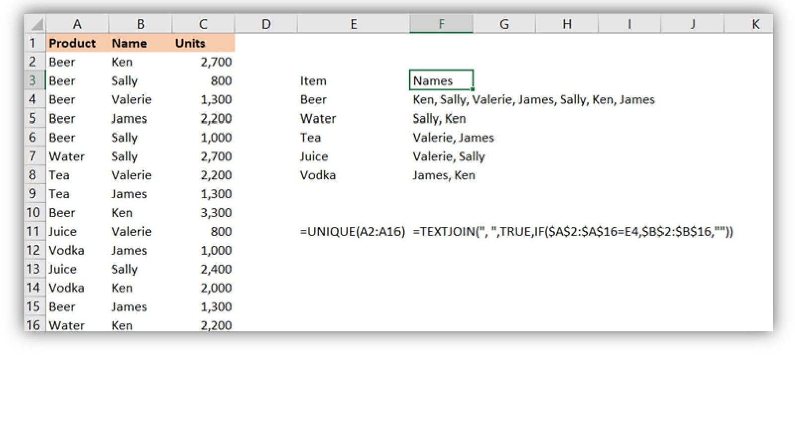
Sometimes dynamic arrays can return an intermittent table which can be aggregated within the same function. One of my favourite use cases of dynamic arrays is to have a conditional TEXTJOIN, and even though the output is in one single cell, a dynamic array is needed when we put an IF formula inside the TEXTJOIN. This same process works in Excel and Sheets, but in the latter, you would need to wrap the entire formula inside ARRAYFORMULA.
This video walks the TEXTJOINIFS process:
Using # notation (Winner Excel)
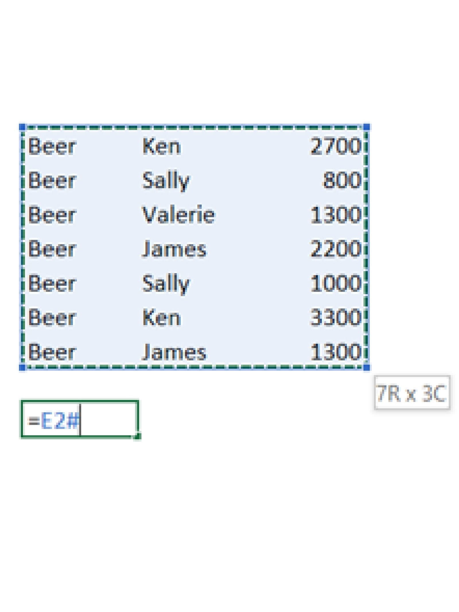
A dynamic array output can be difficult to reference elsewhere, so in Excel, typing the root cell and the # symbol gives you the entire dynamic array (however large that may be). This is useful in data validation ranges or other formulas. In the example below, =E2# (a filter of columns for “beer” currently refers to 7 rows but if the data changes there could be fewer or more rows in future.
Conclusion
Although Excel has a better UI and the # notation is handy, there is no question that Google Sheets’ functions are far more elaborate and flexible, I frequently build spreadsheet solutions in Sheets simply because of its better arrays (usually based on the QUERY function), Excel however has the game changing Power Query which can replicate almost all of these without writing a single formula.
Archive and Knowledge Base
This archive of Excel Community content from the ION platform will allow you to read the content of the articles but the functionality on the pages is limited. The ION search box, tags and navigation buttons on the archived pages will not work. Pages will load more slowly than a live website. You may be able to follow links to other articles but if this does not work, please return to the archive search. You can also search our Knowledge Base for access to all articles, new and archived, organised by topic.
