Excel Tips and Tricks #443 - Next level FILTERing (The FILTER Function)

In previous posts, filters have been covered in some detail, including a recent refresh on the basics of filters and a discussion of advanced filters in the archives. We’ve even covered the Google Sheets FILTER function, which for a time had no equivalent in Excel, but no more. The FILTER function brings the ability to generate a subset of your main listing using complex, multi-level criteria and more dynamic filter options, and is introduced as one of Excel’s dynamic array functions available in Excel for Microsoft 365, Excel 2021 and mobile apps.

How FILTER works

FILTER basically does what it says on the tin – outputs a filtered version of your data.

=FILTER(array, include [,if_empty])

The required inputs are also fairly straightforward – your source array (ie, what you want to filter), and your criteria (ie, what you want to filter on). We’ll come onto the if_empty argument in a bit.

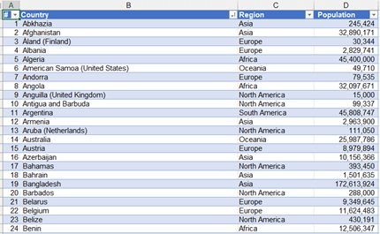
Take a simple scenario – I have a list of countries with their region and population. To manage the list I keep it in alphabetical order, but I also want to be able to view it by population size and/or region without touching the main listing.

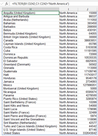
Here, the FILTER function is the answer. On a separate sheet (or indeed, elsewhere on the same sheet), if I want a list of North American countries I just need the formula:

=FILTER(A1:D242,C1:C242="North America")

And hey presto – that’s what we get:

A couple of caveats – you’ll need to apply formatting to the range you expect the data to be returned to (conditional formatting may be your friend here), and the filter won’t return any header rows, so you’ll need to set those up in advance.

Going beyond the basics

It is possible to quite quickly scale up the complexity here, while also improving the functionality. For starters, setting up your ‘master list’ as a Table means the formula cell references are much simpler, and will automatically reflect the size of the table (for more on this, see our recent article on using Excel tables to speed up formulae):

=FILTER(MasterList,MasterList[Region]="North America")

It is also easy to turn this into a dynamic filter, based on a drop-down selection:

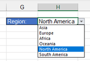
=FILTER(MasterList,MasterList[Region]=$H$2)

This starts to move beyond what can be achieved using standard filter functionality, without having to get into the world of VBA. However, when applying dynamic filters in this way, you need an option for when your drop-down selection is blank, as otherwise by default you get a #CALC error. Which is where ‘if_empty’ comes into play.

In another remarkable ‘does what it says on the tin’ move, ‘if_empty’ tells Excel what to return if your filter criteria returns no results. You may wish to go for the simple “” option, or a “Returned no results” statement, or, as I’ve done in my example, get it to return the full table:

=FILTER(MasterList,MasterList[Region]=$H$2,MasterList)

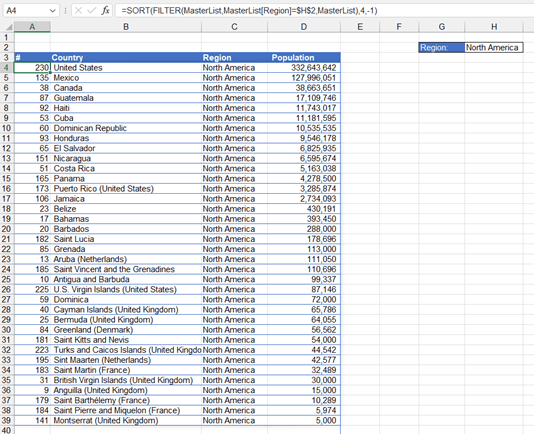
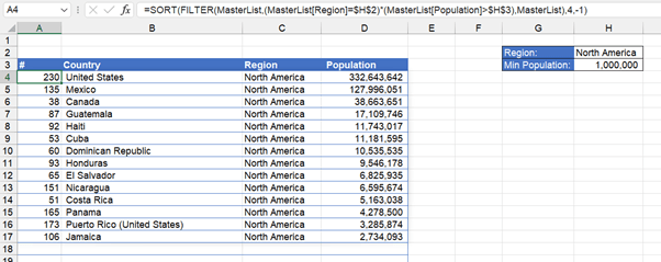
To really nail my example, I want the results sorted by population size. So, I’ve added in a SORT (or you could use SORTBY if you wanted to apply multiple criteria). Throw in some formatting and this is what we get:

=SORT(FILTER(MasterList,MasterList[Region]=$H$2,MasterList),4,-1)

Multiple filter criteria

So far, so good. But what if I need to use multiple criteria in my FILTER? Say I want to add a filter by population size? This is where it is slightly less intuitive, but can take your filter to superpower levels.

Unfortunately, you can’t use operator functions like AND or OR in the FILTER function, but you can apply arithmetic logic to your include parameter. In other words, use * in lieu of AND, and use + in lieu of OR. You can also use parenthesis for different combinations of * and + as required. In this way, you can consider each criteria to return 1 if true, or 0 if false, and the row to be returned by the FILTER function if the result of the equation for the include parameter is not zero. The + option is actually quite powerful given the ability to apply an ‘OR’ logic based on two different columns is not something currently achievable using standard Excel filters.

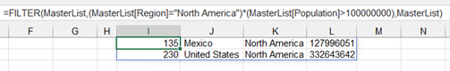
To demonstrate, this, which filters on all countries in North America with a population greater than 100m:

=FILTER(MasterList,(MasterList[Region]="North America") * (MasterList[Population]>100000000),MasterList)

Returns:

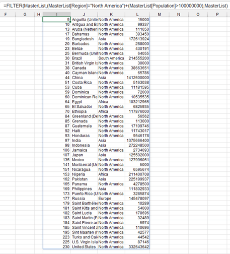
While this, which filters on all countries in North America OR countries with populations greater than 100m:

=FILTER(MasterList,(MasterList[Region]="North America") + (MasterList[Population]>100000000),MasterList)

Returns:

The ability to apply OR logic to filters really does open up a world of new filtering options and solves one of the most common frustrations in using the standard filter tools. However, for our example, AND logic is the way to go – and with another dynamic filter on population, we have a really useful example that can be used as a guide for other similar scenarios.

The joys of FILTER

The FILTER function really comes into play when you want people to have access to explore a data table, but you want to ensure that they don’t start meddling with the raw data. I’m not going to go into edit range permissions (that’s a tip for another day) but if my example was a shared spreadsheet, I could assign different tabs to different regions, and give different people in my team edit access to each tab, while protecting and hiding the Master tab. This would be useful if I had different team members focusing on different geographic regions.

So there we have it. FILTER quite literally takes your filtering to the next level, with more complex filter criteria, the ability to apply filters dynamically, and allowing you to retain control over your master listing. Why not give it a try using the attached example file!