
'How to' series
In this series we will be looking at the Excel tools and techniques that help you accomplish a range of day-to-day Excel tasks more efficiently and effectively.
As part of each article, we will be scouring the extensive Excel Community archive to provide links to additional details and ideas.
Having previously looked at how to enter cell references in formulae using dollar signs to fix all or part of a reference, and the use of Range Names to make formulae easier to enter and understand, this time we will start looking at how the use of Excel Tables can make it quicker to enter Excel formulae.
Tables – not just a pretty format
When Excel Tables were first introduced, many thought that their main purpose was to quickly apply formatting to a range of cells. The presence of the 'Format as Table' command in the Styles section of the Home Ribbon seemed to reinforce this assumption. However, Tables are far more important than that and they can make it quicker and easier to enter better formulae and also make those formulae easier for others to understand in a similar way that we saw with the use of Range Names that we discussed last time.
Referring to Table contents
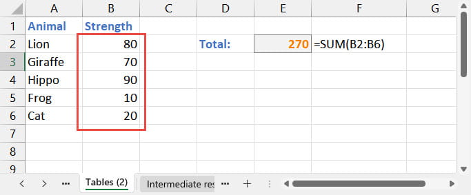
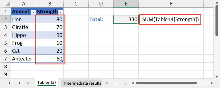
We can demonstrate one of the greatest benefits of arranging data in Tables by using one of the most commonly-used Excel functions: SUM(). If we have a block of cells containing values in one column and we want to include a total of those cells we can use SUM():
If we add a row immediately beneath our range, our SUM() function fails to include it automatically:
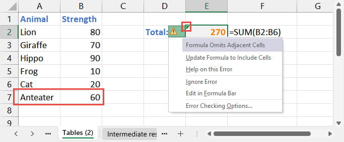
As we can see, our formula now only refers to part of our column, omitting our new row. If turned on, Excel error checking should flag this as a potential problem.
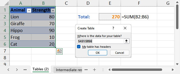
We will go back to our original range and convert it into a Table by clicking a single cell within the range and using one of:
- Insert Ribbon tab, Tables group, Table;
- Home Ribbon tab, Styles group, Format as Table;
- the Control+t keyboard shortcut.
Because our range of cells has been set up without any blank rows or columns, Excel can recognise the entire range of cells that we want to convert into a Table:
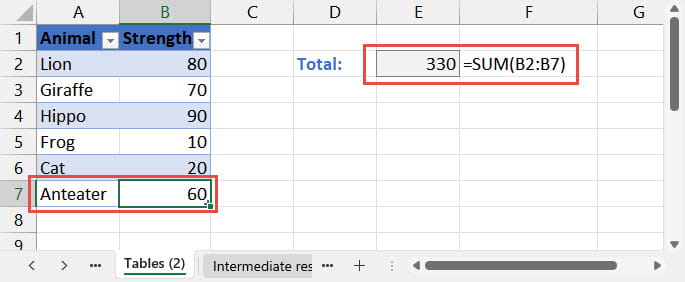
Without making any change to our SUM() formula itself, we will add our anteater line back and see that the reference in our formula now updates automatically to include our new row:
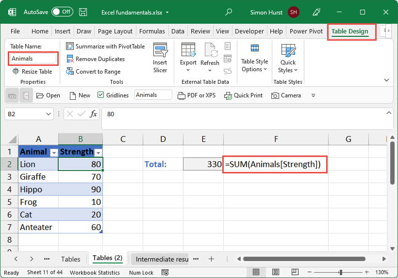
If we recreate our SUM() formula by clicking on B2 and dragging down to B7, now that our range is a Table, we can see another advantage of the use of Tables:
Because we are referring to an entire Table column, our reference uses the Table and column name. We can make this more meaningful by clicking in our Table and using the Table Design contextual Ribbon tab, Properties group, Table name: box, to enter a more descriptive name for our Table:
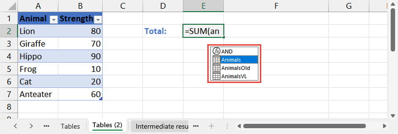
If we need to refer to part of a Table from another worksheet for example, the use of structured references can be quicker than using click and drag to select the required range. When we start typing a Table name as part of a formula, formula AutoComplete is displayed showing Table names as well as function and range names:
Having selected our Table name from our AutoComplete list, we can then type the left square bracket to display a list of column names to choose from:
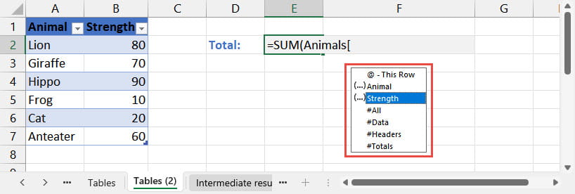
As well as the column names, this list also includes various other elements.
@ is used to refer to 'This Row':
=SUM(Animals[@Strength])
The modifiers preceded by # designate which part of the column to refer to if you want to reference just the header, the totals row, or the whole column including the header and any total. For example, this formula will return just the column header:
=Animals[[#Headers],[Strength]]
Generally, with the exception of just referring to the data in the chosen column, it's usually easier to enter the reference by clicking on the cell rather than typing and using AutoComplete. Excel with then sort out the syntax including the modifier for you.
Absolute relativity
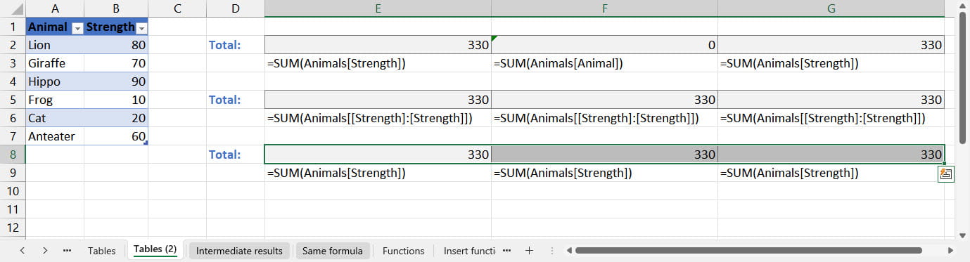
One point to note when creating references to Table columns is that the reference is relative, unlike a Range Name. If we were to copy our =SUM(Animals[Strength]) formula two column to the right, the reference would cycle through our two Table columns. If we want to refer to the Strength column in all three references, we could use the cumbersome workaround of referring to the range of columns from Strength to Strength:
=SUM(Animals[[Strength]:[Strength]])
However, it's often simpler to use the Control+r shortcut to fill right. So, we could just select from our cell containing our formula across to whichever cell we want, and then use Control+r to fill the formula across as in the bottom of our three examples below:
Next time
In the next episode we will look at other ways in which Excel Tables make entering formulae easier and quicker, particularly when including formulae within Tables.
Related links:
Archive and Knowledge Base
This archive of Excel Community content from the ION platform will allow you to read the content of the articles but the functionality on the pages is limited. The ION search box, tags and navigation buttons on the archived pages will not work. Pages will load more slowly than a live website. You may be able to follow links to other articles but if this does not work, please return to the archive search. You can also search our Knowledge Base for access to all articles, new and archived, organised by topic.
