Excel Tips & Tricks #476 - Cross join in Excel using a formula

I put out the following ChatGPT challenge on LinkedIn:

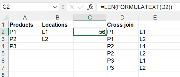
Write a #prompt that will produce a correct answer to this #Excel problem in the picture: create a two-column list of all combinations of products and stores. Specify the Bing mode (Creative to Precise) or the GPT model and temperature.

The resulting table is the same as you would get with a SQL query "SELECT * FROM Products, Locations" which is referred to as an outer join. And indeed, you can do this with Power Query, but queries need to be refreshed, and I wanted a formula.

Nobody was able to craft such a prompt, but two solutions were given by Excel expert Bo Rydobon, who frequently solves LinkedIn Excel challenges. Let's explain his solution for two columns by building from the ground up.

It has always been possible to create a cross-join in a two-way table in Excel by using a classic Ctrl+Shift+Enter array formula such as this:

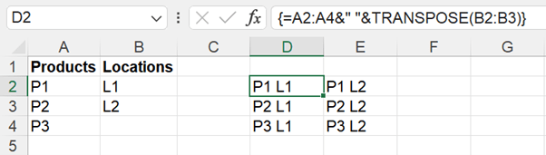
This is not the two-column list I asked for, but it was interesting to me as I had not known at the time of the technique of concatenating a row with a column.

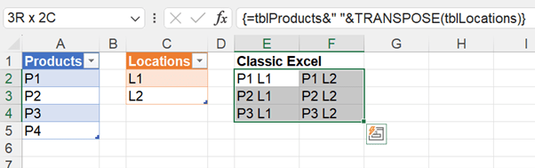
If we convert each column to a separate table, we could use the table column names instead of the cell addresses in the formula. But because we have toselect a fixed output range before pressing Ctrl+Shift+Enter, it will only ever display in the range we have selected, it does not automatically adjust if the number of items in each list changes. In the next screenshot, I added a fourth product.

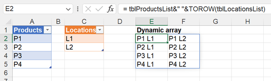
To create a formula that gives a complete cross-join when the number of products or locations changes, we need to use a modern dynamic array formula. An introduction on dynamic arrays has been covered in Tip #437.

Now to convert this two-way table to a pair of columns, we first concatenate the pairs of cells with a distinctive separator such as an underscore, and add a terminating separator at the end such as a pipe symbol.

=CONCAT(tblProductsList&"_"&TOROW(tblLocationsList)&"|")

Gives

P1_L1|P1_L2|P2_L1|P2_L2|P3_L1|P3_L2|P4_L1|P4_L2|

Now all we have to do is split this according to the delimiters we chose:

=TEXTSPLIT(CONCAT(A2:A4&"_"&TOROW(B2:B3)&"|"),"_","|",TRUE)
P1 L1
P1 L2
P2 L1
P2 L2
P3 L1
P3 L2
P4 L1
P4 L2

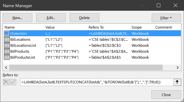
Finally, if you do this more than once in a workbook, why not create a user-defined function to simplify writing it? In the Name Manager, create the name OuterJoin with the following formula:

=LAMBDA(listA,listB,TEXTSPLIT(CONCAT(listA&"_"&TOROW(listB)&"|"),"_","|",TRUE))

And now all you have to enter in the spreadsheet is =OuterJoin(tblProductsList,tblLocationsList)

More examples of using LAMBDA in excel have been covered in Tip #459.