Excel Tip of the Week #437 - Revisiting dynamic arrays

This is an update of our original introduction to the subject from TOTW #327.

What is a dynamic array formula?

In old Excel, array formulas could be used to make formulas that normally only accepted one input instead work with several. There were two key families: Those that were contained in a single cell and which combined the results of the individual formulas back together in some way, and those that spread out over several cells. In either case these formulas only worked if you pressed Ctrl Shift Enter after typing them, and for the multi-cell formulas you needed to pre-select the range that they would live in before entering them, and then couldn’t amend the size of that range afterwards.

This all made for a pretty clunky experience, and old arrays were rightly regarded as a complicated and finicky part of some high-end users’ arsenals only. This all changed however with the introduction of dynamic arrays.

In Excel 365 and later, array calculation is the default. If you provide a formula that expects a single input with a range instead, it will automatically return a range of results, in a process called “spilling”:

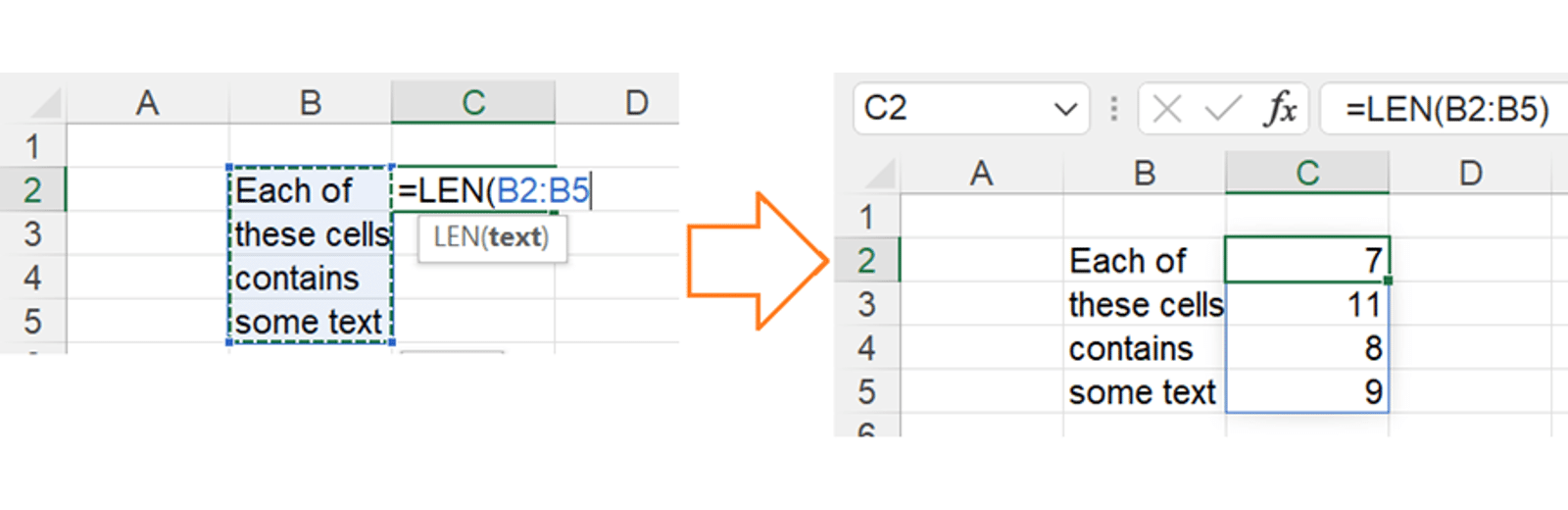
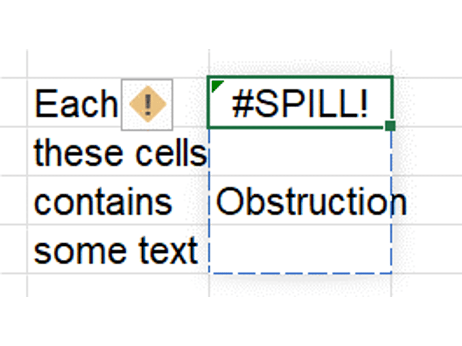
All the cells inside the blue pinline have no formula, but have values which are populated from the anchor cell in C2. This new spilling behaviour does also introduce a new error message if there is something in the way of the spilled output:

And if your cell includes a function that summarises that array into a single result, then it will just work – no special key presses needed:

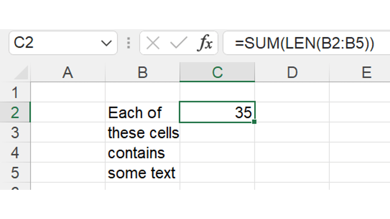
More on this in Simon’s recent article.

Dynamic arrays also introduced a couple of new pieces of Excel formula syntax. Firstly, old Excel would interpret a formula like =A1:A10 – if entered without Ctrl Shift Enter – by using so-called implicit intersection. This meant that it would take the value from A1:A10 that lined up with the formula itself. To emulate this old behaviour, use @ to mark the range:

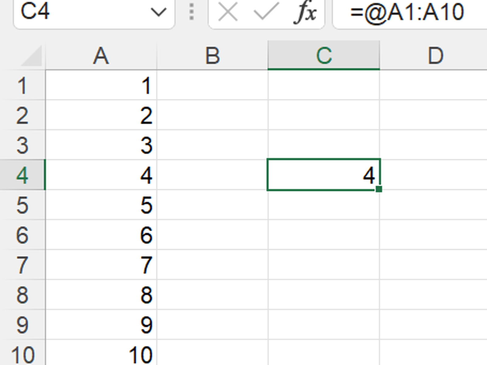
You might find that Excel will automatically insert an @ into some formulas here and there based on its best guess – this is a backwards-compatibility feature and can be turned off.

Much more interesting and useful is the new # operator. When appended to a cell reference, it turns into a reference to the entire range that spills from that cell. This can in turn create a further spilled formula. So take for example this spilled range and a single-cell formula that references it:

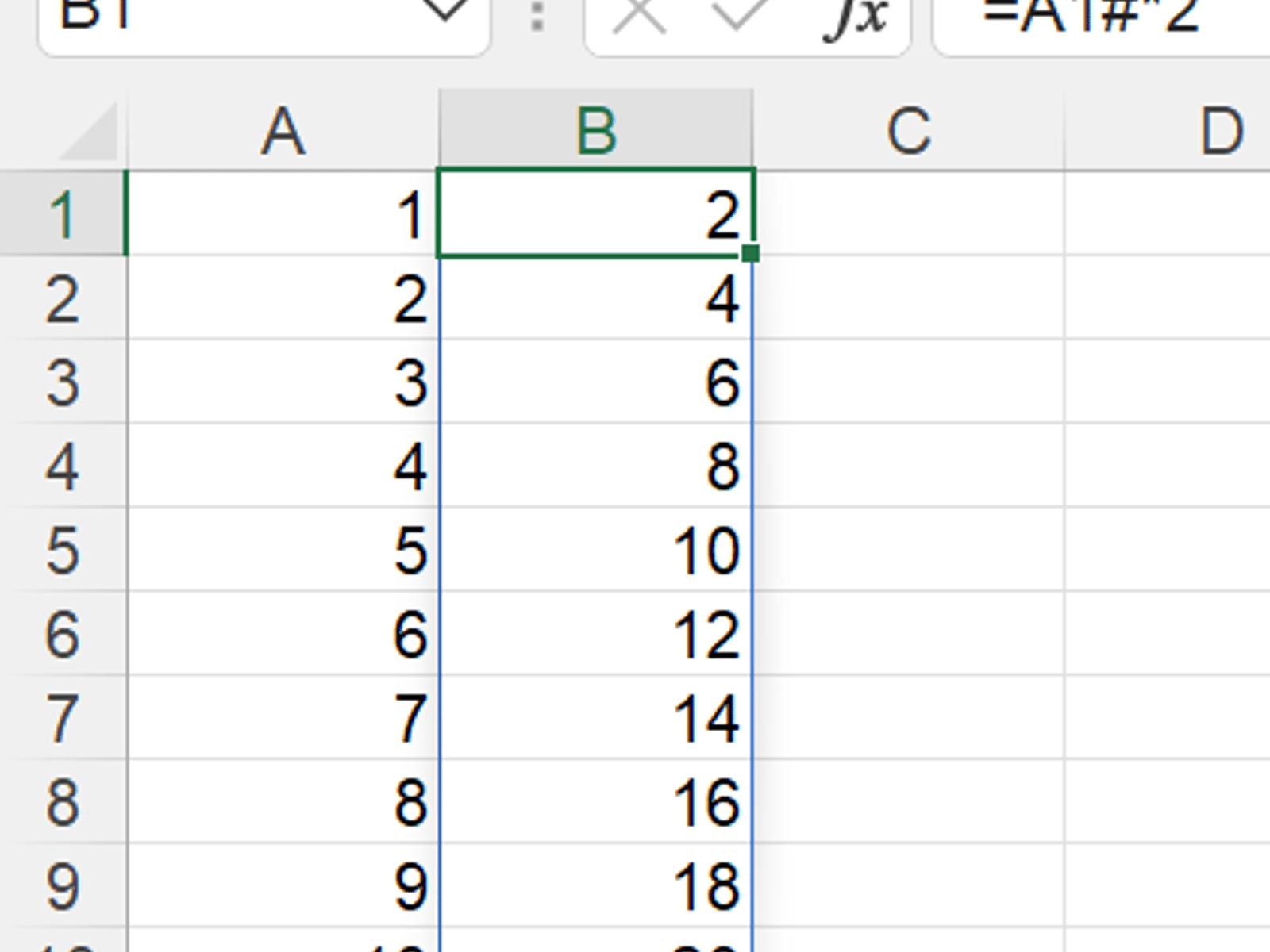
A single # and our function is now yoked to the source array and will grow and shrink as needed to stay matched to it. You can even do a 2D spill by referencing one vertical array and one horizontal array – see below for an example of this.

Dynamic array functions

To supplement the new calculation engine, a bevy of “native spilling” dynamic array functions were introduced. These are designed to return spilled array results and extend what’s possible with Excel formulas.

The key functions are as follows:

SEQUENCE

The simplest and most versatile function in the collection is SEQUENCE, which returns a numeric sequence according to a pattern you specify. The syntax is:

=SEQUENCE(number of rows, number of columns, starting point, step size)

Number of rows is the basic input and the formula will work with just this. For example, =SEQUENCE(5) would return a single column listing the numbers from 1 to 5.

Number of columns can be used instead of number of rows to make a horizontal array, or in combination with it to make a 2D array.

Starting point lets you set a custom starting point for your sequence. If omitted, the sequence will start at 1.

Step size allows you to customise how big a gap there will be between each cell in the sequence output. If omitted the default is again 1. Note that you can use a negative step to create a decreasing sequence.

As well as creating labels or indices for other formulas, SEQUENCE can also be used in combination with other formulas to create clever new functions. For example, =LARGE(range, n) will return the nth-largest item from a range. But replace n with a SEQUENCE(3) function and you can easily return the 3 largest items instead.

RANDARRAY

RANDARRAY is similar to SEQUENCE in that it generates a list of numbers, but instead of a numeric sequence, it generates random numbers. The syntax is:

=RANDARRAY(number of rows, number of columns, minimum, maximum, integer option)

The first two inputs work identically to those for SEQUENCE.
Minimum and maximum set the limits of how large the randomly generated numbers will be.
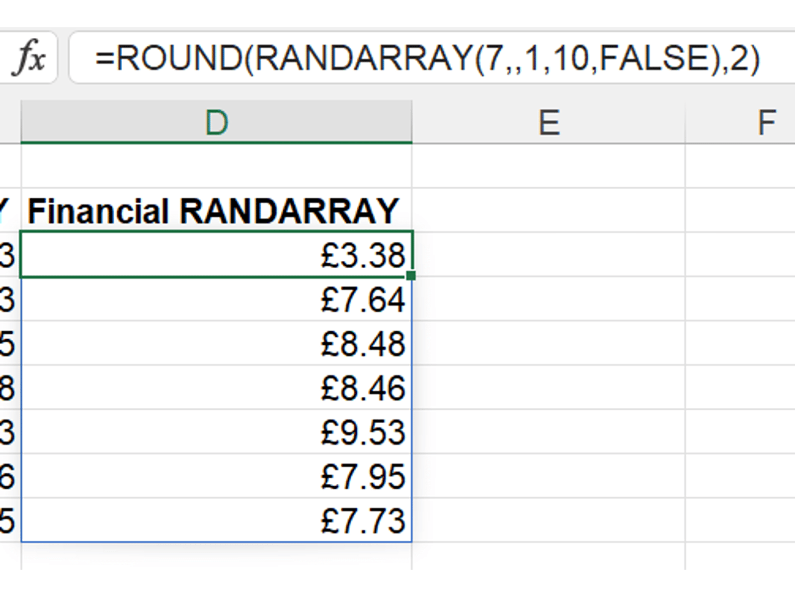
Integer option can be either TRUE, limiting the random numbers to integer values, or FALSE, which will create random numbers out to Excel’s maximum fifteen decimal places. If you want something between these two extremes, such as random numbers with two decimal places to represent dummy transaction amounts, wrap your RANDARRAY in a ROUND function:

UNIQUE

This function returns each distinct, unique value from a range, as a vertical spilled array. The syntax couldn’t be simpler:

 =UNIQUE(range)

There are technically a couple of optional inputs here, for if you want to find unique columns instead of unique rows or if you want to find the rows that appear exactly once instead of one of each unique value. However in almost all circumstances the basic version is all you need.

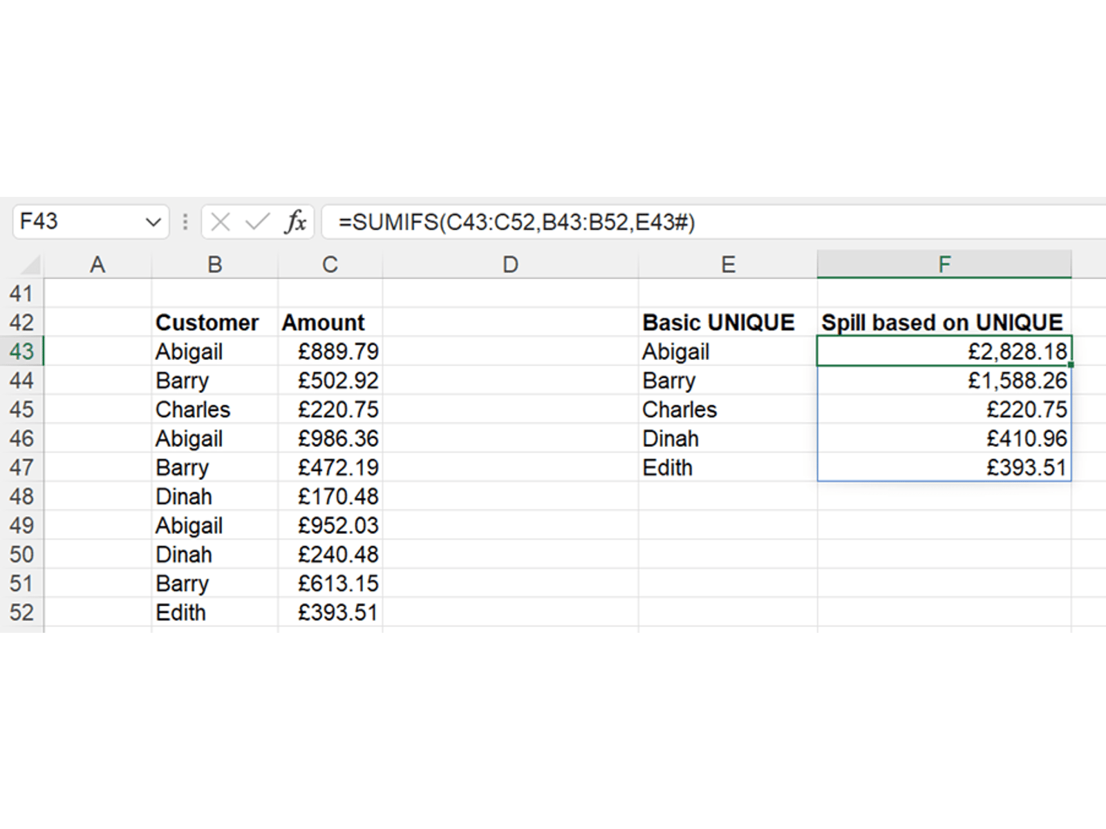
Beyond just making a version of your data with the duplicates removed, UNIQUE is also very handy for making summaries in combination with other functions. For example, here we have used UNIQUE to make a list of the distinct customer names, and then SUMIFS with that array as the condition to make a sum for each. This creates a dynamic and automatically updating version of a sort of PivotTable.

We can take this further if we want to create a true 2D pivot:

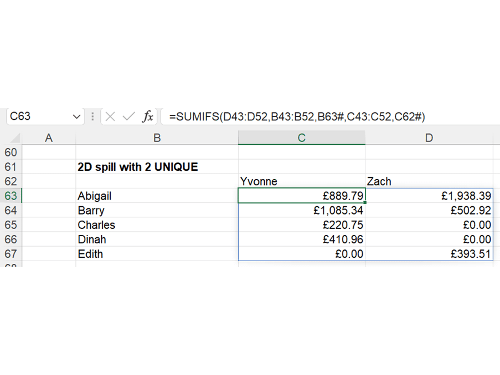
Note that the column header UNIQUE is embedded into honorary spilling function TRANSPOSE, which flips it around into a horizontal array.

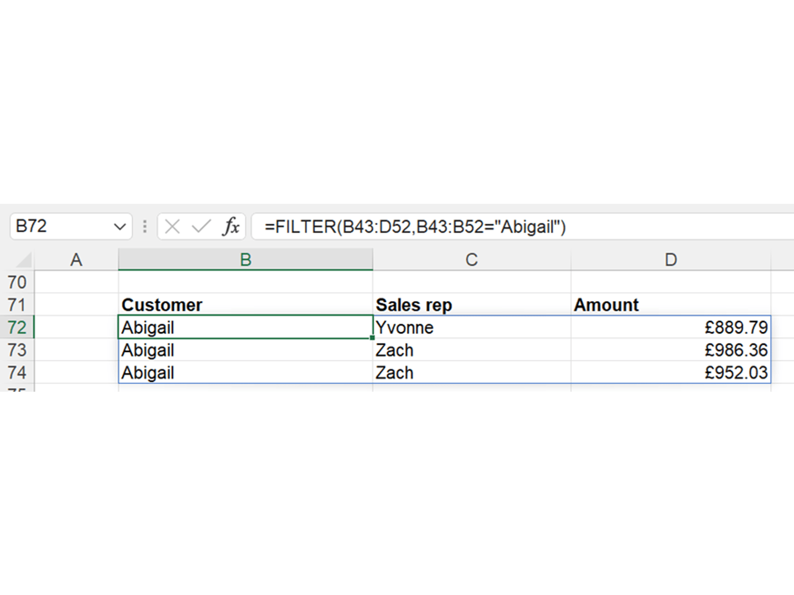
FILTER

This function lets you return an array after filtering it for one or more conditions. The syntax is:

=FILTER(array to filter, one or more conditions, default value)

Array to filter can be any cell range, spilled dynamic range, or formula returning an array which you want to apply a filter to.

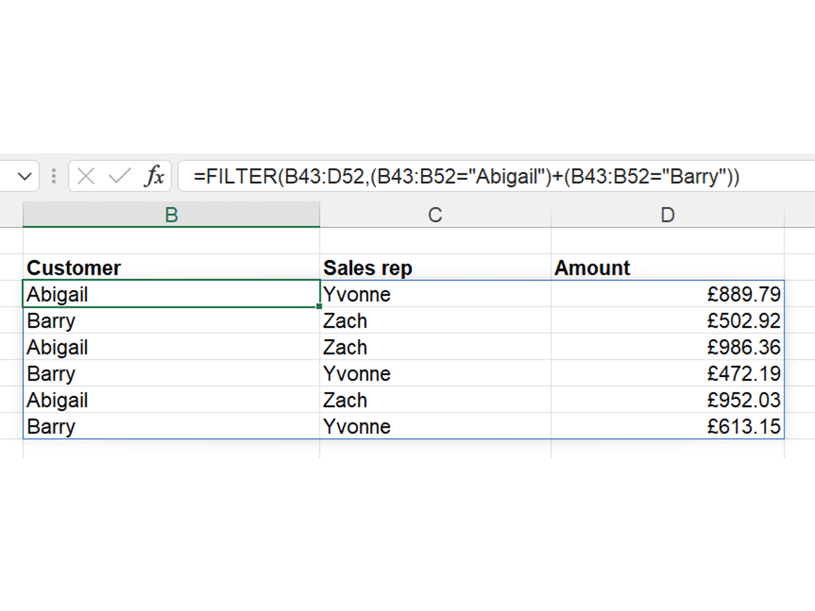
Conditions are entered in the middle input. These have to return Boolean true/false values, e.g. A1:A10=“Apple”, and need to match the size of the array to filter. If you have multiple conditions to apply, these need to be listed in separate sets of brackets and multiplied together (if cumulative) or added (if either/or).

Default value will be used if no rows match the filter – without this a #CALC! error will be shown.

Here’s a simple example of filtering the invoices belonging to the customer Abigail:

Two or more conditions can be combined like so:

SORT, SORTBY

Finally, we have these two functions, which both allow you to sort an array. They are commonly used in conjunction with a UNIQUE or FILTER to provide a sorted output. Let’s take each in turn:

=SORT(array, sort index, sort order, by column)

Array is the range or dynamic array formula that will be sorted. It is the only mandatory input to the function – if you skip the rest SORT will sort the array by the first column, in ascending order.

Sort index is a number that you can use to indicate if you want to sort by a column other than the first.

Sort order can either be 1 to sort in ascending order (the default), or -1 to sort in descending order.

By column is a Boolean input – use TRUE or leave blank to sort by column, or use FALSE if you want to sort by row (i.e. rearrange the array horizontally instead of the usual vertically)

Here’s an example SORT which sorts our invoice table into descending order of size:

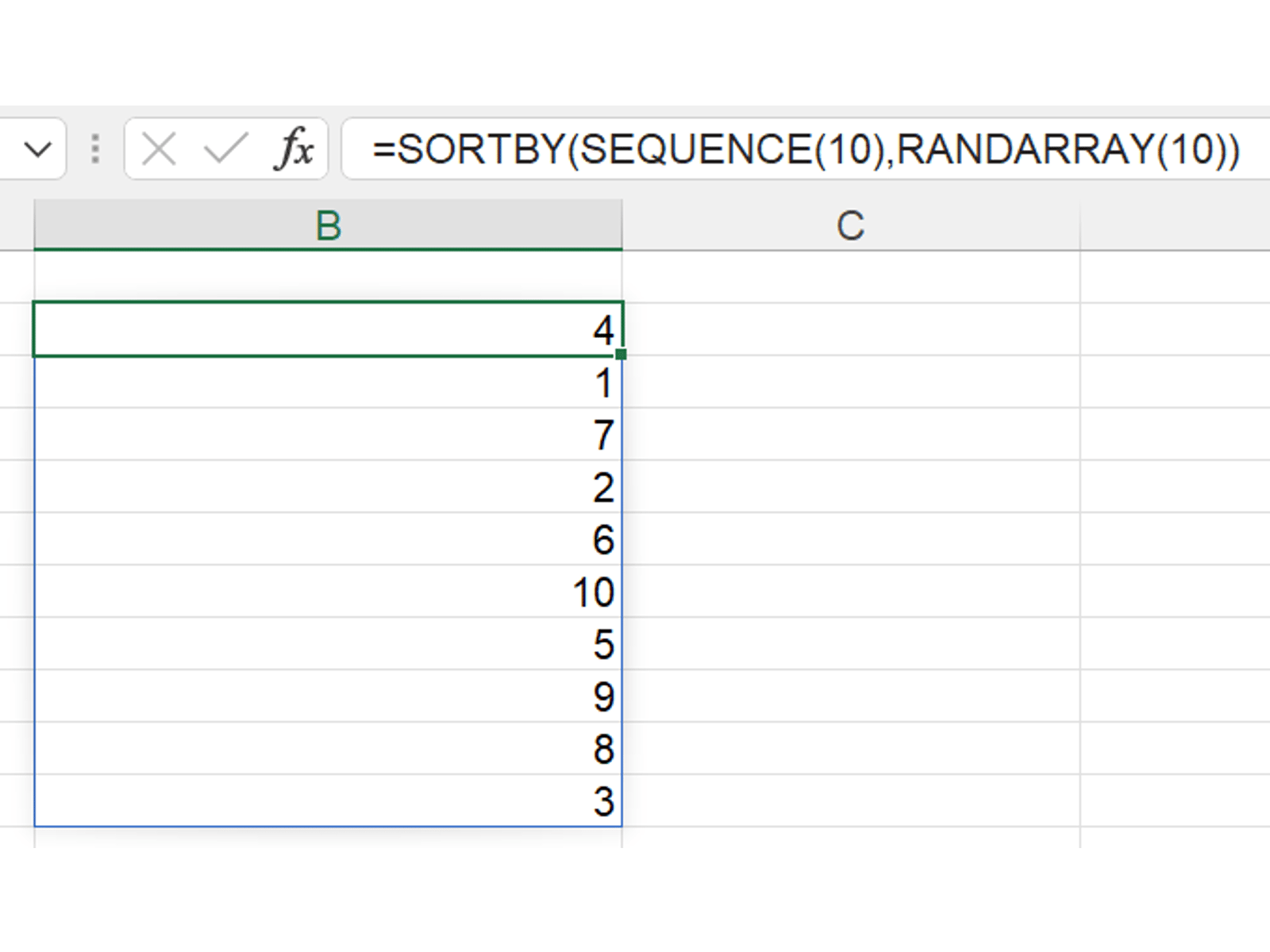
Finally, we have SORTBY. This is very similar to SORT in theory in that it rearranges an array, but the difference is that SORT can only use the contents of that array to sort the data, whereas SORTBY can sort one array by reference to another external one. This is very useful for sorting smaller sections of an array, or for randomising data. The syntax is:

=SORTBY(array, by array, sort order)

Array is, as before, the array to be sorted.

By array is the array to be used for the sorting order; it must be of the same height as the main array. Essentially SORTBY acts like the two arrays are in alignment and sorts the “by array” in order, then outputs the resulting order for the main array.

Sort order is the same as for SORT – 1 or omitted for ascending order, -1 for descending.

Note that the function does technically allow you to specify multiple pairs of “by array” and “sort order” inputs; you could use this to sort by one ordering and then another for tied items, etc.

Here’s an example of using SORTBY to “sort” an array by a RANDARRAY of the same size, the end result of which is to randomise the data:

There are plenty of things covered in this post, so don’t forget to check out the accompanying file for examples of everything in action! 

Previous post – Trimming excess spaces redux
TOTW index
Next time – Power Query – Creating custom functions!