Dynamic Arrays – it's not just about the new functions and spilling

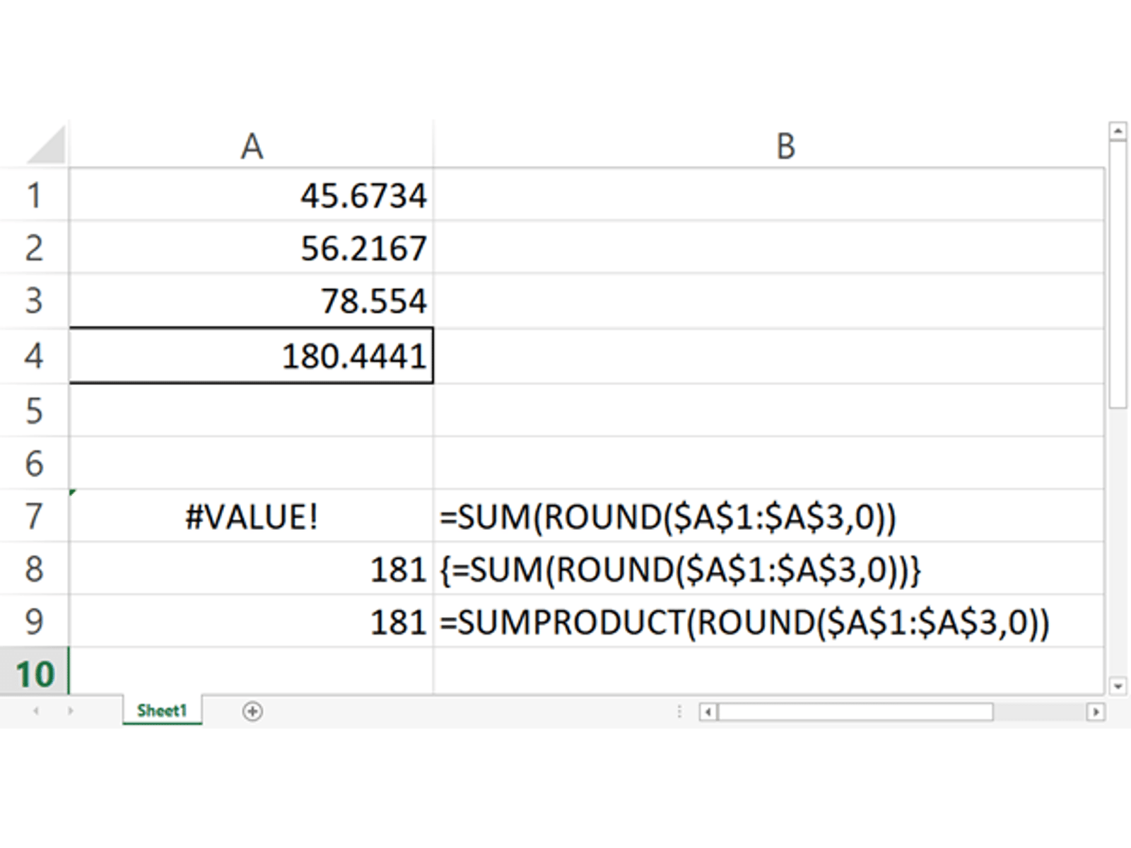
In addition to this change, several new functions were introduced to take advantage of the new capability. However, at least equally important is the ability to process arrays within a formula in a single cell. This is not completely new. Before Dynamic Arrays, the Control+Shift+Enter key combination could be used to create an array formula, or the SUMPRODUCT() function could be used as a 'wrapper' for formulae that used arrays. For example, the following formula used to result in a #VALUE! error as the ROUND() function couldn't cope with a range of cells, rather than an individual value:

=ROUND($A$1:$A$3,0)

Since the introduction of Dynamic Arrays, this formula would spill down to the two cells beneath the actual formula cell to display three individual results. If your intention is to calculate the total of the rounded values, then you could try wrapping your ROUND() formula in a SUM() function:

=SUM(ROUND($A$1:$A$3,0))

Again, before Dynamic Arrays this would generate a #VALUE! error. To make it work, you would have to change it to an array formula, either by saving it using Control+Shift+Enter or by using SUMPRODUCT():

=SUMPRODUCT(ROUND(($A$1:$A$3,0))

In our new era of Dynamic Arrays, we don't even really have to think about whether our formula includes an array or not, but instead just type our formula as 'normal':

=SUM(ROUND($A$1:$A$3,0))

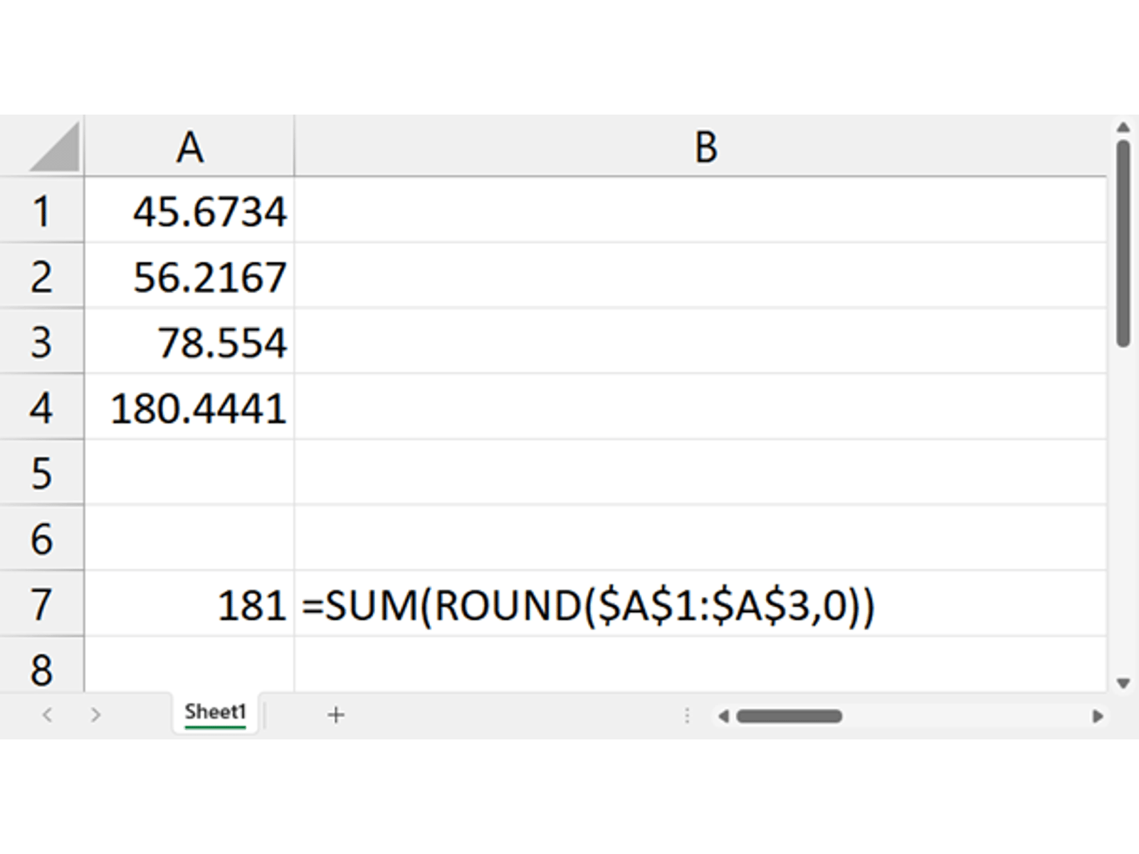
In effect, our Dynamic Array is spilled, and then recombined by SUM(), within our single cell.

Before we look at the advantages, it's worth pointing out that there are consequences for backward compatibility. If we were to use an earlier version of Excel to open a spreadsheet containing:

=SUM(ROUND($A$1:$A$3,0))

Excel would convert our formula to an array formula:

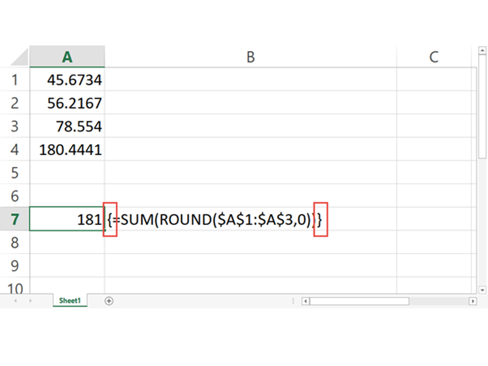
One of the drawbacks of 'old' array formulae is that, unless you always save them using the Control+Shift+Enter key combination, they will revert to a normal formula when edited – even if no change is made.

The complexity and fragility of formulae that use Control+Shift+Enter has tended to how often they are used. Although using SUMPRODUCT() addresses the fragility concern, it does still add a layer of complexity and requires specific knowledge of what the function can do and how to use it. In a Dynamic Array world, people will be able to create formulae that use arrays without needing to worry about whether the function that they are using can cope with arrays or not.

Let's have a look at a practical application of this. One of my support clients recently asked if I could come up with a concise way to check whether a product code was in the correct format. They needed to identify any codes that were not in the format AAA999 where A is an upper-case alphabetical character and 9 is a number from 0 to 9. The number check is less of an issue as we can just use the ISNUMBER() function to check the three rightmost characters in the cell in one go:

=ISNUMBER(VALUE(RIGHT(A1,3)))

For the alphabetical test, it is less obvious how we can test without extracting each character and testing it individually. This would be a bit cumbersome, as we would need to create three separate formulae, each of which would need to check that the individual character was not 'before' the letter upper-case A or after the upper-case Z:

=AND(CODE(LEFT(A7,1))>=CODE("A"),CODE(LEFT(A7,1))<=CODE("Z"))

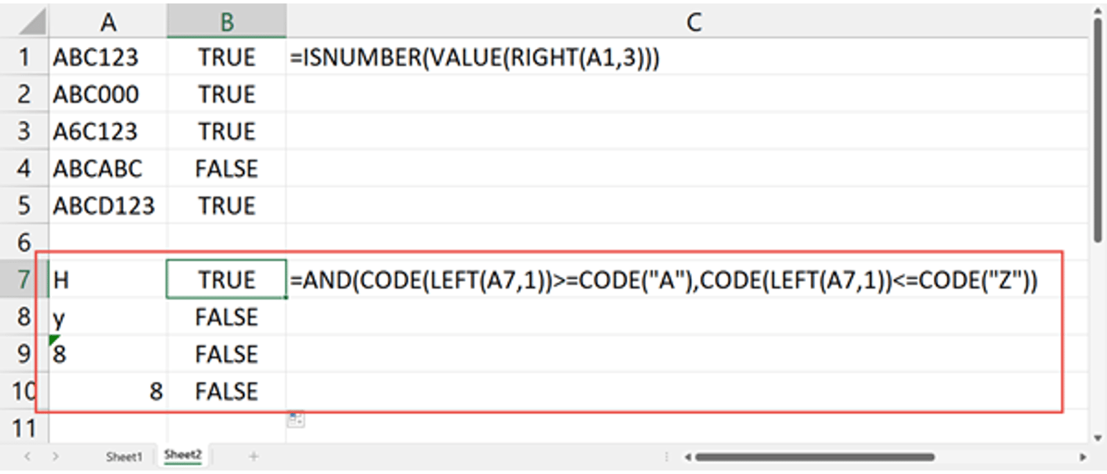
To ensure that only upper-case, alphabetical characters pass our test, we have converted our characters to their corresponding ASCII codes using the CODE() function. We would need to test each of our three characters separately and combine the result using AND().

Using an array, we can come up with a formula that texts all three characters in one go, by using the MIN() and MAX() functions to check whether any one of the three characters is less than A or greater than Z:

=AND(MIN(CODE(MID(A1,{1,2,3},1)))>=CODE("A"),MAX(CODE(MID(A1,{1,2,3},1)))<=CODE("Z"))

We have adapted our single cell formula by using MID() rather than LEFT() and returning an array of the first three characters by setting the second argument of MID() – the starting position – to 1, 2 and 3. Note that to indicate we want to use a list of values, we enclose our 1,2,3 in braces by typing the braces (not by using Control+Shift+Enter).

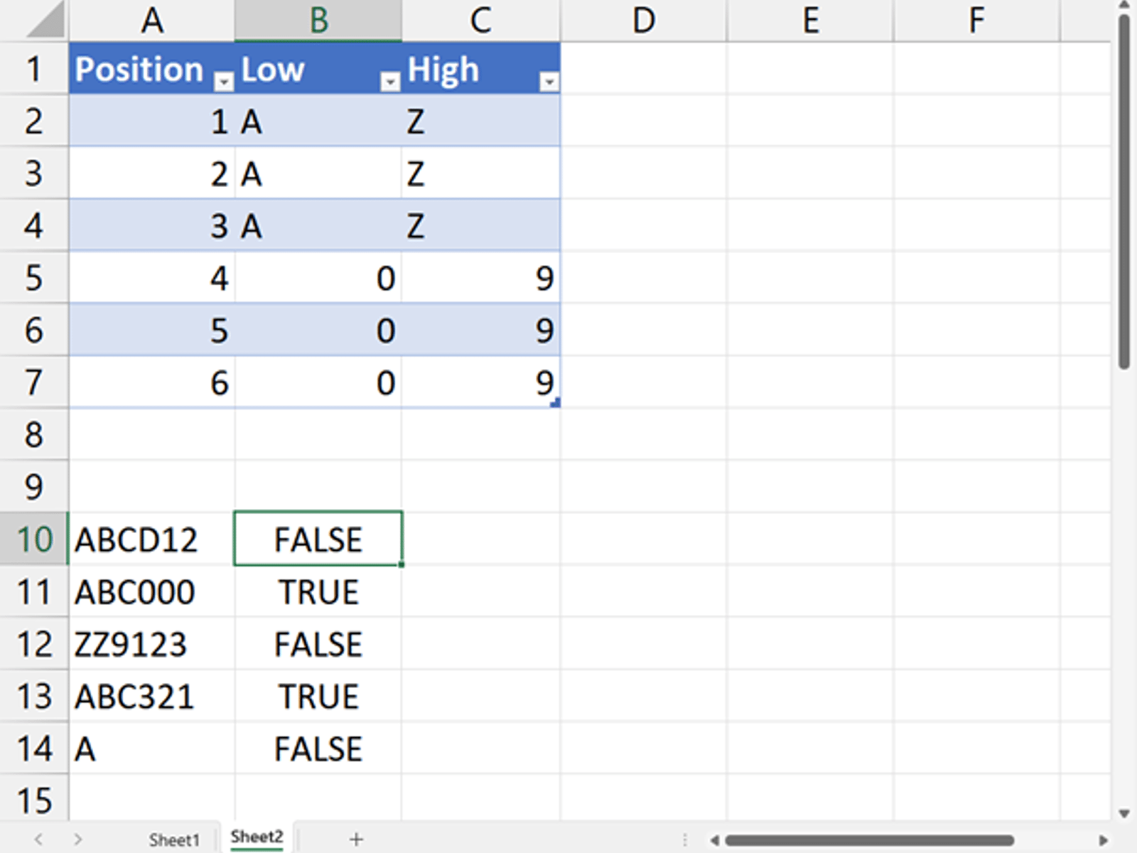
The main part of our validation formula just compares the ASCII code values of the character in each position indexed by the Position column against the ASCII code value of the corresponding characters in the Low and High columns:

=AND(CODE(MID(A10,tblMask[Position],1))>=CODE(tblMask[Low]),CODE(MID(A10,tblMask[Position],1))<=CODE(tblMask[High]))

There is a complication. If the number of characters in a cell is less than the maximum position in our list, then our formula will return an error, as the MID() function will be starting beyond the end of the available text. To avoid this, we will incorporate our check on the length of the code in an IF() statement that will ensure the rest of the check only takes place if the length of our code is equal to the highest value in our Position column:

=IF(LEN(A10)=MAX(tblMask[Position]),AND(CODE(MID(A10,tblMask[Position],1))>=CODE(tblMask[Low]),CODE(MID(A10,tblMask[Position],1))<=CODE(tblMask[High])),FALSE)

Although this example does demonstrate some useful techniques and concepts, I can't help feeling that there must be an easier way. If you know one (apart from using a database rather than a spreadsheet in the first place) please let us know at excel@icaew.com.