Dynamic Arrays and Charts – bigger and better Excel dashboards await

Introduction

This time last month we posted an article about the new Ctrl+Shift+V Paste Special keyboard shortcut with the slightly tongue-in-cheek headline: Rapid Microsoft reaction to keyboard shortcut article – Ctrl+Shift+V . In the article, we claimed that an earlier Excel Community post had triggered Microsoft’s decision to introduce the new keyboard shortcut. Whilst it would be nice to believe that the community had had that much influence, the fact that the preview release of the new shortcut came within hours of the article being posted suggested that coincidence was a more likely explanation. However, just over six weeks ago, another community article looked at the latest functions that had been released to work with Dynamic Arrays. As part of this article, we mentioned some shortcomings in Dynamic Arrays that hadn’t been addressed. One of these was the inability to base charts directly on Dynamic Arrays in a way that would ensure the chart would be automatically updated when the dimensions of the array changed:

“However, when Dynamic Arrays were first introduced, there were some important restrictions to their capabilities. One of these was the inability to include Dynamic Array formulae in an Excel Table. This meant that there was no simple way to, for example, use a Dynamic Array as the source for an Excel Chart so that it would adjust automatically if the dimensions of the Dynamic Array changed, in the same way that linking a chart to an Excel Table would.”

Still not quite a Table

This time last month we posted an article about the new Ctrl+Shift+V Paste Special keyboard shortcut with the slightly tongue-in-cheek headline: Rapid Microsoft reaction to keyboard shortcut article – Ctrl+Shift+V . In the article, we claimed that an earlier Excel Community post had triggered Microsoft’s decision to introduce the new keyboard shortcut. Whilst it would be nice to believe that the community had had that much influence, the fact that the preview release of the new shortcut came within hours of the article being posted suggested that coincidence was a more likely explanation. However, just over six weeks ago, another community article looked at the latest functions that had been released to work with Dynamic Arrays. As part of this article, we mentioned some shortcomings in Dynamic Arrays that hadn’t been addressed. One of these was the inability to base charts directly on Dynamic Arrays in a way that would ensure the chart would be automatically updated when the dimensions of the array changed:

“However, when Dynamic Arrays were first introduced, there were some important restrictions to their capabilities. One of these was the inability to include Dynamic Array formulae in an Excel Table. This meant that there was no simple way to, for example, use a Dynamic Array as the source for an Excel Chart so that it would adjust automatically if the dimensions of the Dynamic Array changed, in the same way that linking a chart to an Excel Table would.”

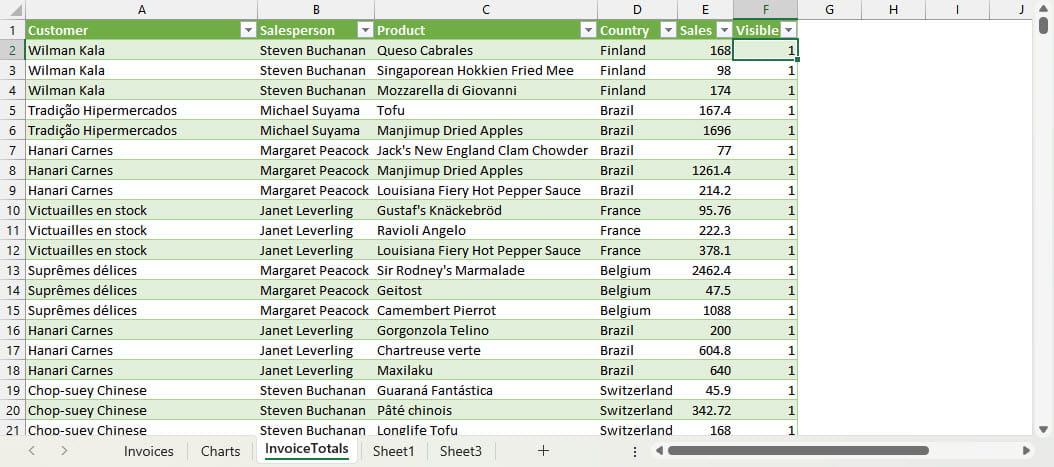
In this example, we have used the UNIQUE() function to extract lists of Product and Salesperson details from our single Invoices Table. We can then use SUMIFS() in an adjacent column, referring to the UNIQUE() Dynamic Array formula with the # operator, to create our summary totals:

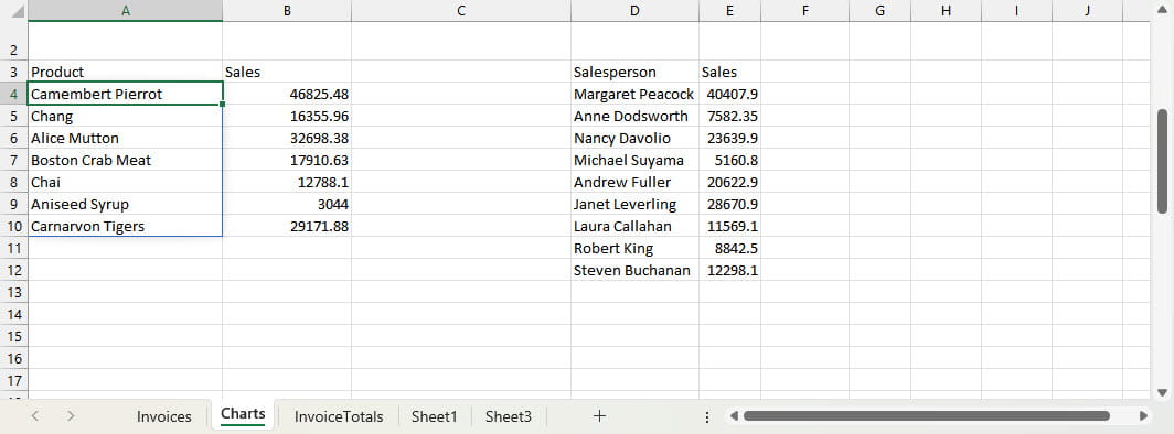
Cell A4 contains the formula:

=UNIQUE(InvoiceTotals[Product])

Cell B4 contains the formula:

=SUMIFS(InvoiceTotals[Sales],InvoiceTotals[Product],A4#)

For our Salesperson array, we use the same formula, but replace the reference to the [Product] column with a reference to the [Salesperson] column.

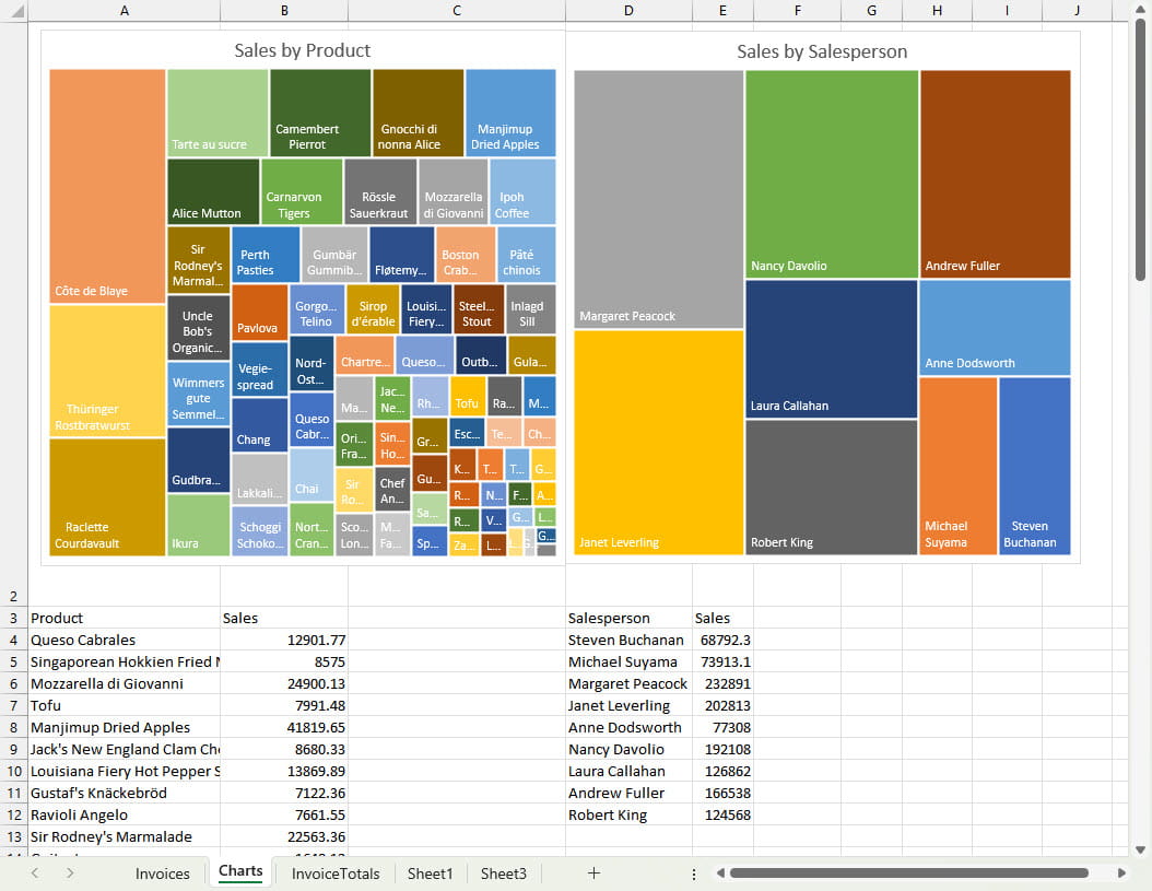
We now create our Treemap charts based on these two Dynamic Arrays and, because of the latest enhancement, this reference will now adapt as the dimensions of the arrays change. We have put the arrays and charts on the same worksheet just for demonstration purposes:

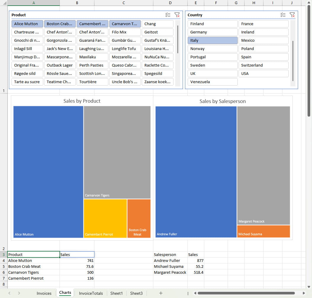
The final step is to add Slicers based on our InvoiceTotals Table. We have one remaining problem that I am indebted to an excellent article by Mark at ExcelOffTheGrid for solving. The Slicer will happily filter the Table on which both of our arrays are based. However, filtering a Table just hides the rows that are filtered out, and our arrays will still refer to the whole Table and will be unchanged by the Slicer. For this reason, we have added a column to the Table that will contain a value of 1 for the visible, non-filtered out, rows and 0 for those that are filtered out. As the ExcelOffTheGrid article sets out, there are two functions that can do this: SUBTOTAL() and AGGREGATE(), both of which will include items in a total if they are visible and exclude them if they are not. We have chosen to use AGGREGATE() and to count non-blank cells (aggregate function type: 3) that are not hidden (aggregate option: 5). We do this referring to the Sales total cell in the current row of the Table:

=AGGREGATE(3,5,[@Sales])

Given that we are aggregating the count of non-blank cells for a single cell, the answer will either be 1 or 0. This means that we can add this as a filter to both of our arrays so that they only return values that have passed through our filter:

Cell A4 contains the formula:

=UNIQUE(FILTER(InvoiceTotals[Product],InvoiceTotals[Visible]))

We have added the FILTER() function, with the criterion set to the [Visible] column value to each formula.

Cell B4 contains the formula:

=SUMIFS(InvoiceTotals[Sales],InvoiceTotals[Product],A4#,InvoiceTotals[Visible],1)

This time we have added a second criterion to the SUMIFS() function to refer to our [Visible] column.

Obviously, we would do the same for our Salesperson array columns.

Now, when we choose values from either Slicer, the rows that are visible in our InvoiceTotals Table will change accordingly. Our Dynamic Arrays will also change and, in an edition of Excel that has the charts enhancement implemented, our charts will also change:

Can you do better?

This is one of those occasions when, although inordinately pleased with having come up with a solution, I can’t help wondering whether there is another very obvious and much simpler solution. If you know of one, please let us know: excel@icaew.com .

Related links

• Charting with Dynamic Arrays
• Dynamic Arrays – still one leg short of a table?
• Dynamic Arrays - limitations of #
• Accountants' guide to Excel - from PivotTable to dashboard