With the addition of so many new, dynamic functions in Excel in recent years, it would be easy to think that some of the more ‘traditional’ functions have had their day. Some, however, still bring huge value to our modelling work despite their old age.

INDEX is one of those functions. INDEX returns the value found at a specific position inside a range. You tell Excel which row to go to, which column to go to, or both, and Excel gives you the value sitting at that intersection.

And INDEX has a few extra features that may surprise you. Let’s take a look.

The anatomy of INDEX

The most common INDEX syntax is:

=INDEX(array,row_num,[column_num])

• array is the range or array of values you want to return from.
• row_num is the row position inside that array.
• column_num is the column position inside that array.

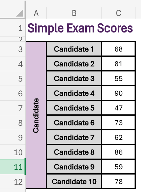
The grid above uses C3:C12 for exam scores by candidate, with candidates 1 to 10 listed down the side. If we want Candidate 7’s result, the formula is

=INDEX(C3:C12,7)

Read that formula from left to right: use the score range, then move to the seventh row. The returned value is the score at that position (62).

Returning from a two-dimensional table

INDEX is often introduced with a single column or single row, but it becomes much more powerful with a two-dimensional grid.

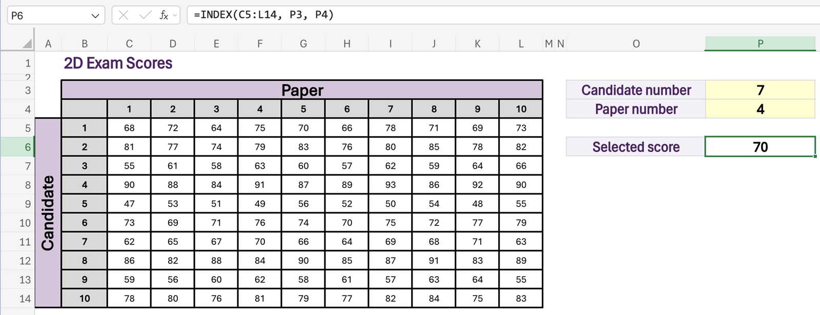
In our exam results example above, both directions matter. The row number identifies the candidate number (the row). The column number identifies the paper (the column). The value returned is the specified candidate’s score in that paper.

That is why this data set works well for INDEX. The row and column numbers are not arbitrary; they mean something. Candidate 7 and Paper 4 are natural positions in the range we reference in the first part of the INDEX function.

=INDEX(C5:L14,7,4)

This returns Candidate 7’s score in Paper 4.

Using zero to return a whole row or column

Most users first learn INDEX as a way to return one value. However, INDEX can also return an entire row or an entire column.

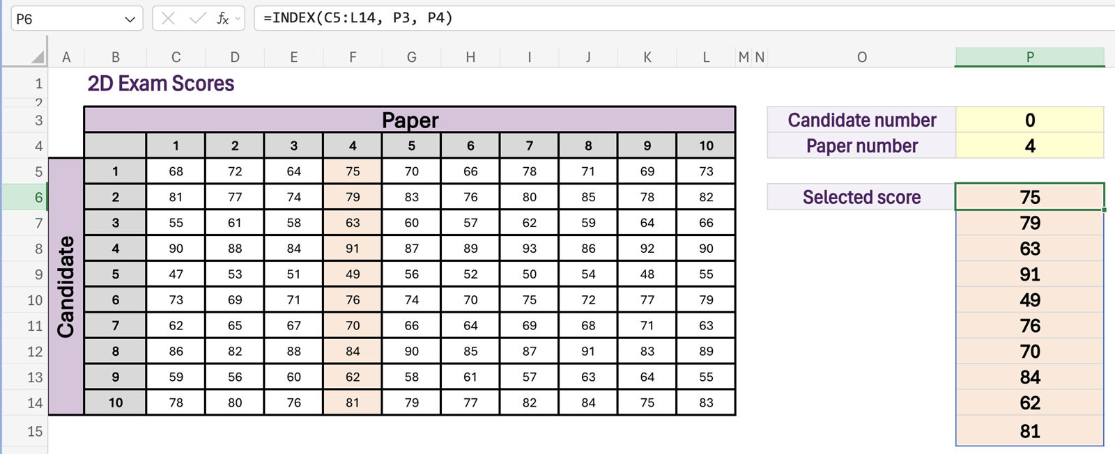
If the row argument (the candidate number) is zero, INDEX returns the whole column you specify. For the example in the screenshot above:

=INDEX(C5:L14,0,4)

This returns every candidate’s score for Paper 4.

In modern Excel, that result spills down from P6 into the cells below. That makes the zero argument a neat way to extract a complete set of results from our starting range or array.

The same idea works in the other direction. If the column argument is zero, INDEX returns the whole row you specify.

The second INDEX syntax: choosing between areas

There are actually two optional forms of syntax for INDEX. The one we have mainly used is the array form:

=INDEX(array,row_num,[column_num])

The less commonly used form is:

=INDEX(reference,row_num,[column_num],[area_num])

The extra area_num argument lets INDEX choose between multiple separate ranges. In the supporting workbook on the AreaSyntax tab, each school has its own 10 x 10 exam score grid. Those separate school grids can be treated as areas within our INDEX function.

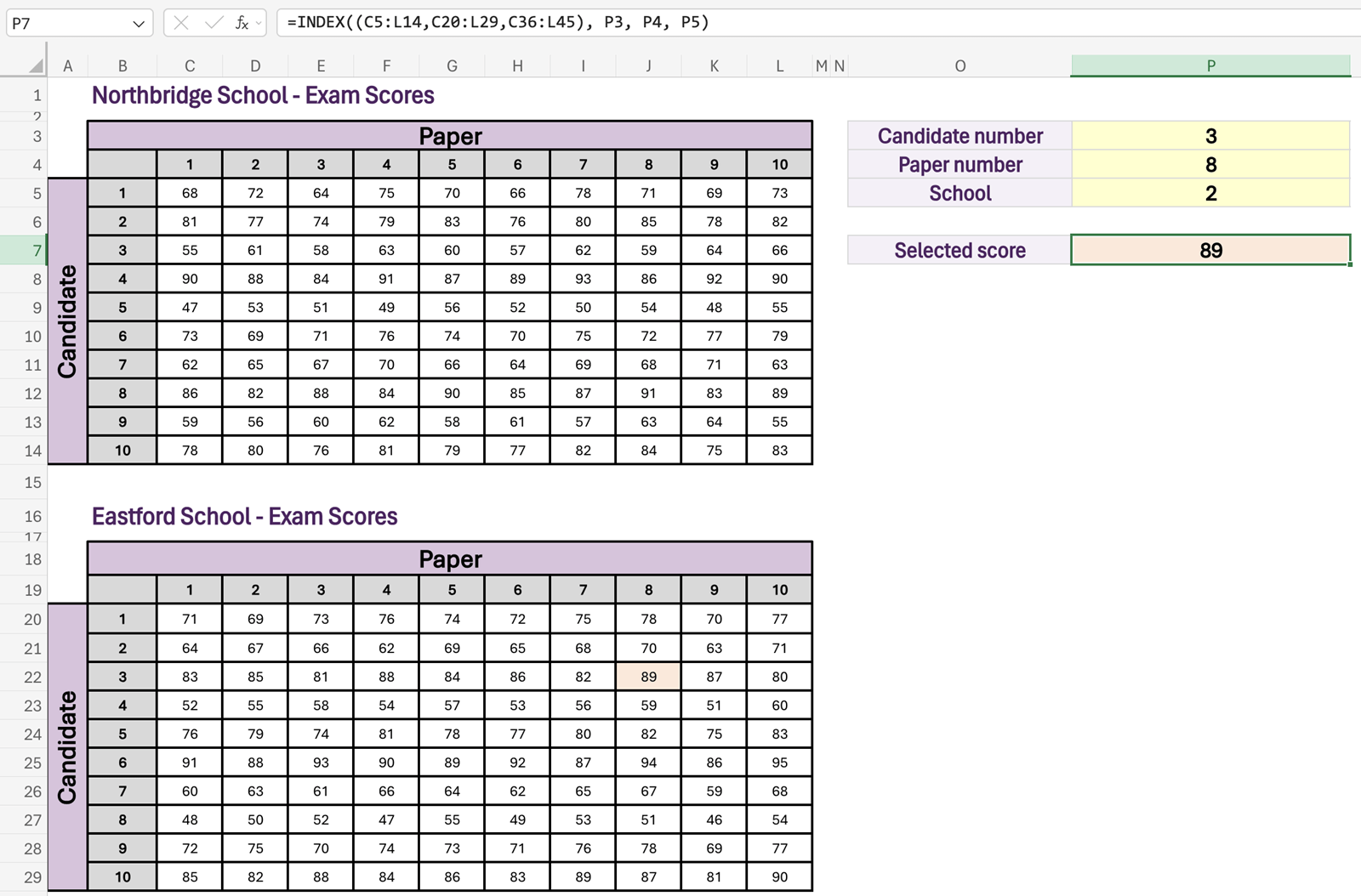
=INDEX((C5:L14,C20:L29,C36:L45), P3, P4, P5)

This tells Excel to use the second area, then return row 3 and column 8 from that area. In plain English: return Candidate 3’s Paper 8 score from Eastford School.

Most users will not need the area syntax, but it is useful to know it exists. It also reinforces the core concept: INDEX is still returning from a position. The area argument simply adds one more coordinate: which grid should Excel actually use?

Where XMATCH fits in

On its own, INDEX works when you already know the position you want. In this article, that position is obvious because candidate numbers and paper numbers align to the position numbers from 1 to 10.

In many workbooks, however, you may not know the position. You might know a name, a date or a code, and need Excel to work out where that item appears. Historically, the classic pairing was INDEX and MATCH: MATCH found the position, and INDEX returned the result at that position.

Today, I would usually use XMATCH rather than MATCH because it is more flexible, but the idea is identical: XMATCH finds where something is; INDEX returns what sits in that position.

That distinction is worth understanding even if many would turn to XLOOKUP today. XLOOKUP combines the search and return steps in one function. INDEX keeps the retrieval step separate.