
There’s little doubt that the introduction of Dynamic Arrays has been one of the most revolutionary changes in Excel in recent years. Like Power Query, Dynamic Arrays change the way in which we approach a significant range of different spreadsheet requirements. However, when Dynamic Arrays were first introduced, there were some important restrictions to their capabilities. One of these was the inability to include Dynamic Array formulae in an Excel Table. This meant that there was no simple way to, for example, use a Dynamic Array as the source for an Excel Chart so that it would adjust automatically if the dimensions of the Dynamic Array changed, in the same way that linking a chart to an Excel Table would. As usual with Excel, there is a workaround, in this case using a Range Name to hold the reference to the Dynamic Array:
Within the last few months, a new set of Dynamic Array functions has been added to Excel. Currently these are only available on the Insider Beta update channel, but they are sufficiently significant that, even if you don’t yet have access to them at the moment, it’s worth being prepared for their arrival in your edition of Excel. There is the proviso that things can change between the release to the Beta Channel and the eventual general release.
We are going to look at these new functions and how they can help with the Dynamic Array/Table problem, although without yet providing a solution to the specific problem of dynamic Excel charts.
The new Dynamic Array functions allow Dynamic Arrays to be ‘shaped’ by changing the number of rows or columns or by combining multiple arrays. We have already covered the two functions that combine arrays, VSTACK() and HSTACK(), in a previous article:
This is a quick guide to the other shaping functions that are on their way.
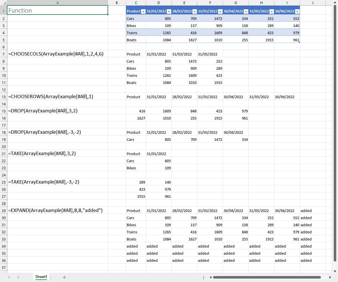
- CHOOSECOLS() and CHOOSEROWS(), as their name suggests, allow you to choose columns or rows from an array by specifying the index number of the row or column that you want to include in your new array or formula.
- DROP() and TAKE() allow you to create a subset of an array by removing or including rows and/or columns from the beginning or end of an array. Positive numbers of rows or columns work from the start of the array and negative numbers from the end. You can think of this as including or excluding rows and columns from the top left-hand corner of an array for positive numbers or from the bottom right-hand corner for negative numbers.
- EXPAND() adds rows or columns to an existing array by allowing you to specify the new, larger, number of rows and/or columns and the content to be included in the additional cells:
There are other new shaping functions for more specific tasks. TOROW() and TOCOL() allow a two dimensional array to be rearranged as a single row or column, with an argument provided to specify whether to read through the original data by row or by column:
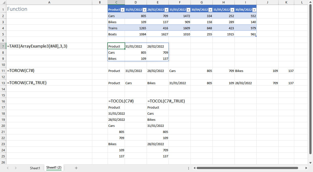
Note that in the above example we have used the TAKE() function to just include the top left-hand corner 3 rows and 3 columns. We have then referred to that array in our TOROW() and TOCOL() functions by referring to the top left-hand corner cell of our new array and adding the # suffix:
=TOROW(C7#)
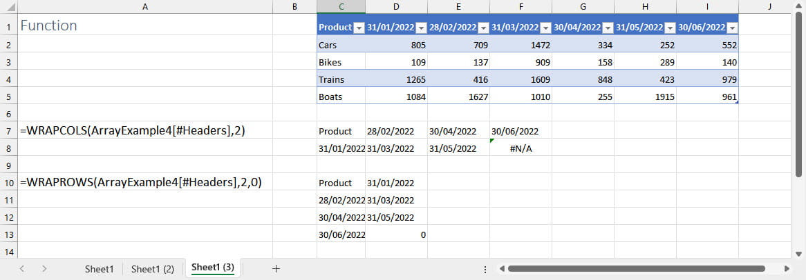
Before looking at some of the practical applications of these new functions, for completeness we will also provide examples of two further Dynamic Array shaping functions: WRAPROWS() and WRAPCOLS(): These functions wrap a single row or column into multiple rows or columns. Each function allows you to specify the one-dimensional range and the number of rows or columns to arrange it across. The WRAPROWS() example demonstrates the use of the third argument to specify a value to pad any empty cells that result:
As we saw with the TOROW() and TOCOL() examples, the use of the # suffix extends a reference to all the cells that the formula in a cell spills into. This can be used in combination with CHOOSECOLS() to allow a reference to a Dynamic Array to work in a similar way to a Table column, and automatically adjust as the number of rows changes.
One of the simplest demonstrations of the benefit of using an Excel Table is a to use SUM() to total a Table column rather than a simple range of cells. If we add a row to the Table, our SUM() formula will include the new row, whereas a SUM() formula that refers to a range of cells outside of a Table will not adjust to the addition of a value in the cell beneath the existing range.
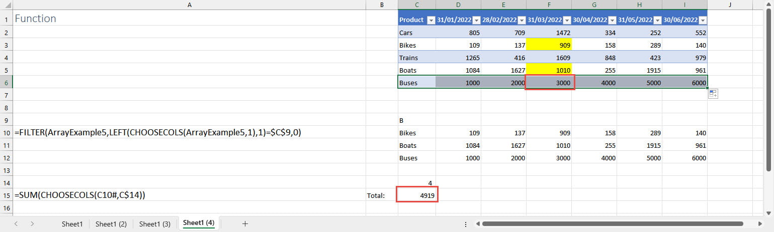
In the following example, we have used a Dynamic Array formula to return all the rows from our Table where the text in the first column starts with the single letter entered in cell C9. We have then calculated a total of one of the columns in this array. We return the array by referring to the top left-hand corner cell of our array and using the #suffix. We have specified the column to use by entering the index number in cell C14:
=SUM(CHOOSECOLS(C10#,C$14))
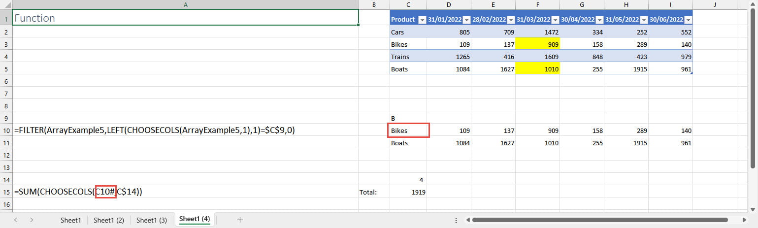
If we had another B word to our Table, we see that our total updates automatically to include the new value added to the fourth column:
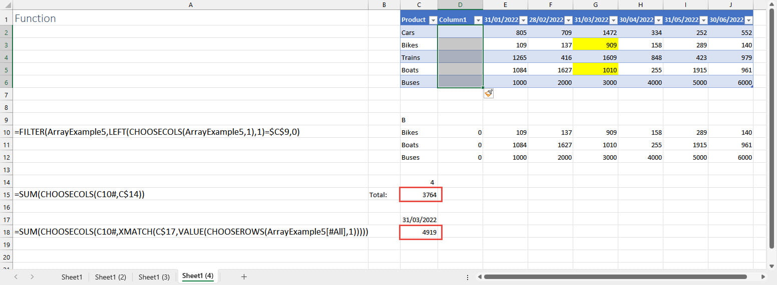
Of course, the reference to a fixed column number might be a concern. If we were to add a Table column to the left of column 4, our total would be adding up a different column. We could overcome this by calculating our column index number using the XMATCH() function:
=SUM(CHOOSECOLS(C10#,XMATCH(C$17,VALUE
(CHOOSEROWS(ArrayExample5[#All],1)))))
Note that Table column headers are treated as text so, to make our XMATCH() function work with a date entered in cell C17, we need to use the VALUE() function to convert our text date to a real date:
Once they become more generally available, we will look at some further practical applications of these new functions.
Join the Excel Community
Do you use Excel in your organisation? Are you using it to its maximum potential? Develop your skills and minimise spreadsheet risk with our Excel resources. Membership is open to everyone - non ICAEW members are also welcome to join.

Archive and Knowledge Base
This archive of Excel Community content from the ION platform will allow you to read the content of the articles but the functionality on the pages is limited. The ION search box, tags and navigation buttons on the archived pages will not work. Pages will load more slowly than a live website. You may be able to follow links to other articles but if this does not work, please return to the archive search. You can also search our Knowledge Base for access to all articles, new and archived, organised by topic.