Power Query versus VBA – part 1

I've often wondered whether, had Power Query had been developed before Excel macros, if there would have been much use for Visual Basic for Applications (VBA) code. Of course, this is a bit of an exaggeration, but to illustrate the point I thought I'd take a recent Tip of the Week post on the use of VBA code to calculate stamp duty and see whether Power Query could provide an alternative method. Before we start, and to possibly prevent you wasting your time reading this article, one big compromise that we need to make when using Power Query is the need to refresh our calculation when any of the inputs change. When using cell-based formulae in Excel we are used to calculations happening automatically whenever the value in a relevant cell is changed. Although a Power Query query can be set to update at timed intervals, the refresh cannot be triggered directly by the input values changing (unless you use VBA!).

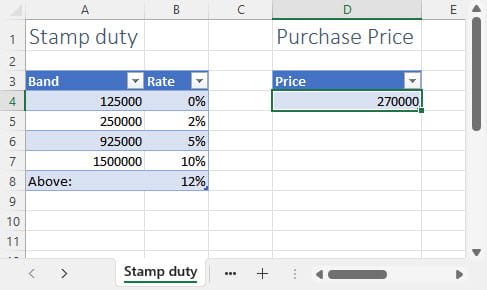
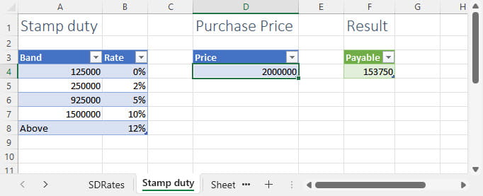
So, for the few of you who are still reading having overcome any negative feelings about the refresh operation, this shows how we will set up our table containing the stamp duty bands and rates. There are a few ways in which we could bring in our property purchase value. We could put the value in a cell that has had a Range Name allocated to it and then link to the Range Name in Power Query. Alternatively, we could put our value in a (very small) Excel Table and use the Drill Down capability to extract our purchase value. We will be using this, second, method:

As usual with Power Query projects we start by clicking in our Table and using the Data Ribbon tab, Get & Transform Data group, From Sheet (previously known as From Table/Range) command to load our Table into the Power Query editor. There are many ways in which we could carry out the necessary calculations and we haven't necessarily chosen the most concise or elegant method, but we have hopefully used a method that is relatively clear and makes the resulting calculations easy to understand and check.

We'll start with the easier Table first and just load the Price Table into the editor. Once we have loaded the Table, we can just right-click on our value in our one and only row and use Drill Down to turn our Table into a single value with the name Price.

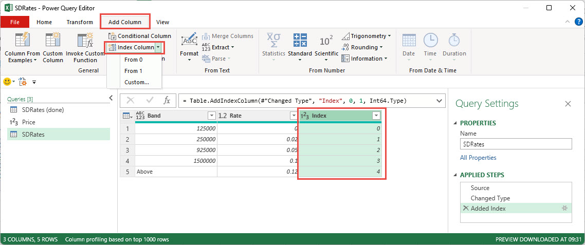
Next, we will calculate some of the values that we are going to be using in the Stamp Duty Table itself. One of these calculations will require us to refer to a value in a different row of our Table so, to facilitate this, we will add an index to our table using the Add Column Ribbon tab, General group, Index Column command. The dropdown for this command gives options to allow us to start the Index from 0 or 1, or to create a custom index by specifying the starting number and increment to use. For our purposes, it doesn't really matter whether we start our index with 0 or 1, so we'll just click on the command itself, rather than using the dropdown, to create a default index column, starting with 0:

We are going to use this new Index column to add a column to our table that will show the end value of the previous band. We use the Index value to allow one row to refer to another row. This is the custom formula that we enter using the Custom Column command:

= #"Added Index" [Band]{[Index]-1}

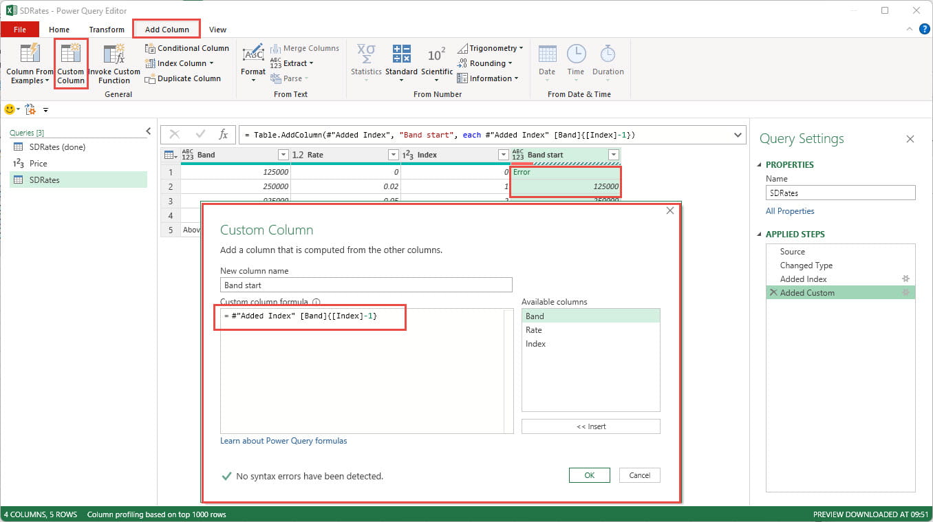
Although the references to the [Band] and [Index] columns can be entered by double-clicking each one in the 'Available columns' list, the rest of the formula needs explanation:

#"Added Index" – this is a reference to a table: in this case, the table created by the query step Added Index which is the previous step in our list of APPLIED STEPS. Note the # sign and use of double-quotes.

Having defined the table that we are working with, we can extract a value from a particular column. In our case we use [Band] to refer to the Band column. However, we don't want to use the value from the current row of the Band column but instead we want to use the value in the previous row. We can specify which row to use by entering the number of the row between braces {} immediately after the column reference. To refer to the previous row, we use our Index column and subtract 1:

[Band]{[Index]-1}

This works for all our rows except the first one because clearly the first row doesn't have a previous row, so our Index calculation returns an error. We could handle this with a conditional formula, but it is easier to use Power Query's version of Excel's IFERROR() function: 'try…otherwise':

=try #"Added Index" [Band]{[Index]-1} otherwise 0

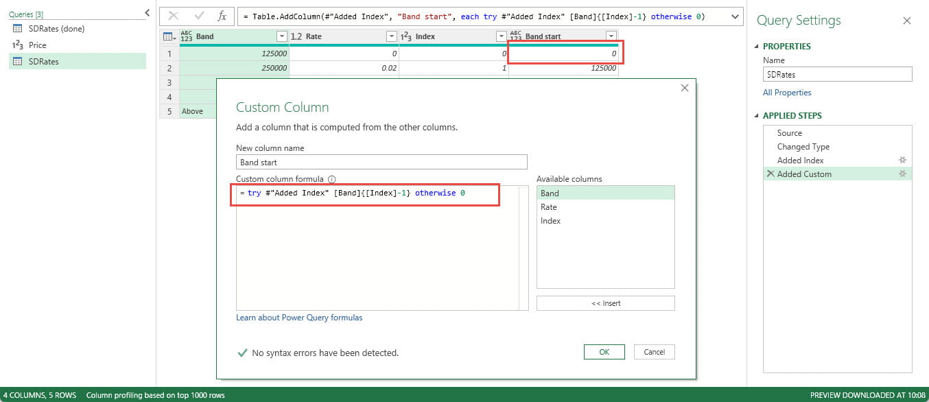
Power Query will 'try' our formula and, if it doesn't return an error, use our formula. However, if it does return an error, it will use the value we specify after 'otherwise'. In our case, 0.

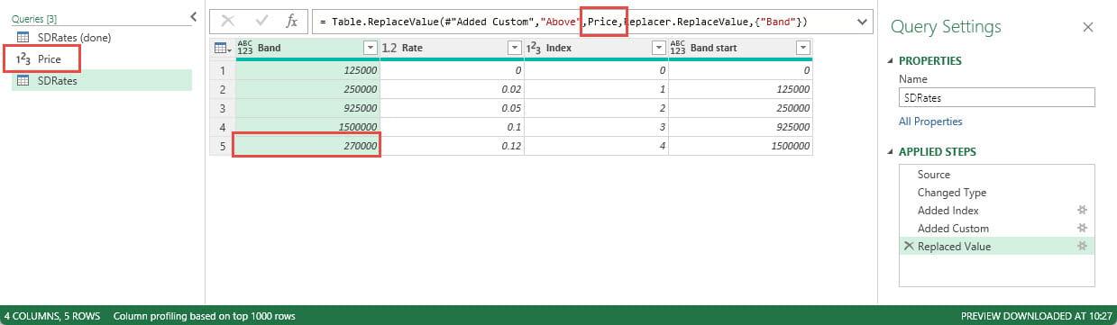
The next issue we need to address is the final band which applies to all values above our previous band end. The formula that we will be using to calculate the actual stamp duty payable would seem to depend on this band being, in effect, infinite. We have entered the text 'Above' in our source table and we could just click on this value and use the Home Ribbon tab, Transform group, Replace Values command to replace it with some implausibly high value. However, what we actually need this band to be is the lower of infinity and the purchase price of our property. Accordingly, we will use Replace Values and just enter Price to create the step we need, then edit the formula for that step to refer to our Price value by removing the double quotes that Power Query will use to identify the text value we have entered:

= Table.ReplaceValue(#"Added Custom","Above","Price",Replacer.ReplaceValue,{"Band"})

= Table.ReplaceValue(#"Added Custom","Above",Price,Replacer.ReplaceValue,{"Band"}):

Next, we want to create a column to hold the total value of stamp duty payable for each band which we will name: Cumulative. This requires another Custom column, but this time it simply uses our existing column values and some maths:

=([Band]-[Band start])*[Rate]

To calculate the amount of stamp duty due for each band, we will use a conditional formula. Often, the easiest way to get the syntax correct is to use the Conditional Column command in the General group of the Add Column Ribbon tab. Where the Conditional Column can't cope with some of the content, such as using greater than and less than rather than equals and not equals, and referring to our Price value, we can just edit the resulting formula afterwards. Our formula needs to check whether our Price is higher than the Band value. If it is, we just use the Cumulative amount for that band that we have already calculated. If it isn't higher, we multiply the difference between the Band start value and the Price, by the Rate.

This is the Add Conditional Column dialog with the values and operators that we will need to edit highlighted:

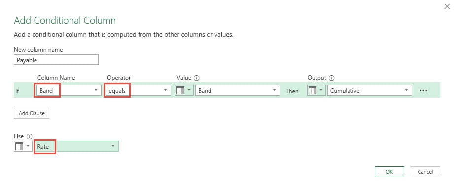
This is the resulting formula before editing:

= Table.AddColumn(#"Added Custom1", "Payable", each if [Band] = [Band] then [Cumulative] else [Rate])

Then once edited:

= Table.AddColumn(#"Added Custom1", "Payable", each if Price >= [Band] then [Cumulative] else [Rate] * (Price-[Band start]))< /blockquote>

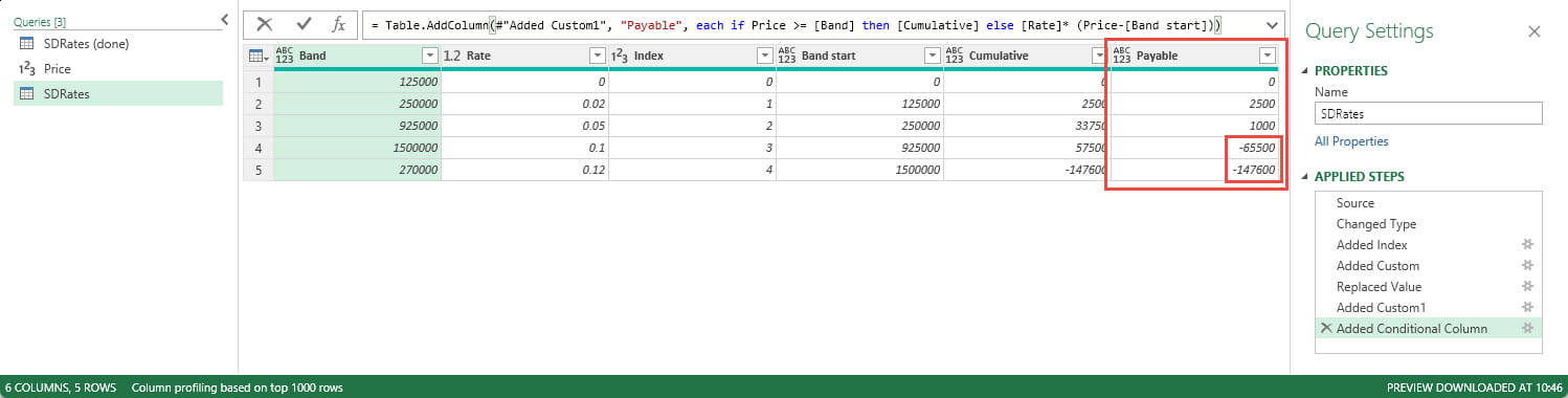
We are not quite finished yet because, where the Band start is higher than the Price, our calculation will return a negative value. We just need to filter our Payable column to only include positive values. This leaves us with just the stamp duty payable values we need for each applicable band:

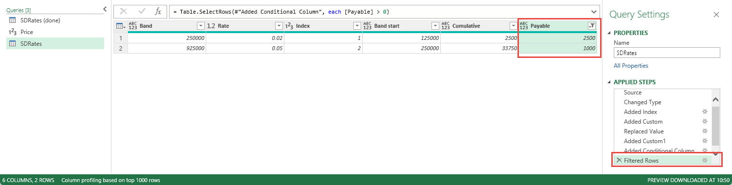
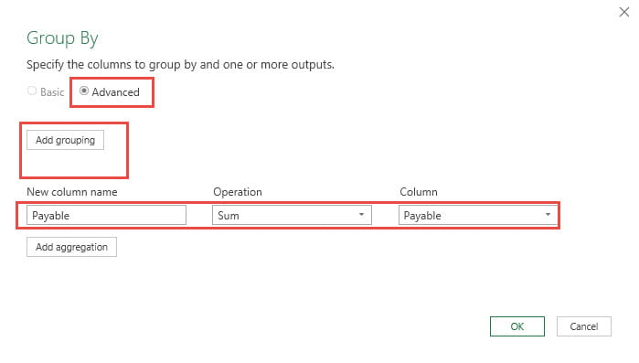
To turn this into a single value of stamp duty payable, we can use the Transform Ribbon tab, Group By command and use the Advanced option to delete the default grouping and set our Column name to Payable; our Operation to Sum and our Column to Payable:

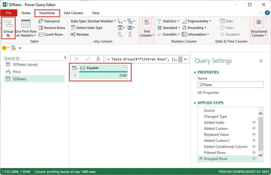
Grouping without using a group will just total all our rows into a single row and, because we have only specified one aggregation, a single column:

Our Power Query process would then require extensive testing with test Purchase Price values, looking particularly at the boundaries between rates and values in excess of the highest band specified:

In part 2, we will examine some advantages of using Power Query to perform calculations and how it could be used more generally to create a more modular approach to the construction of spreadsheets.