Ungrouping Groups

Sometimes, you want to “regenerate” the underlying data, so analysis may be performed at a record-by-record level. The aim of this article is to provide ideas regarding how Power Query / Get & Transform might assist.

Let’s take a generic example. Imagine the following had been written in shorthand:

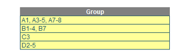
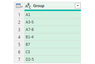
The above was a summary of the following:

Therefore, for the first row you had a value for Group “A” (which could be any text), one [1], then the integer values three [3] through five [5] (i.e. 3, 4, 5) and then seven [7] and eight [8].

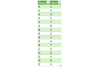
The aim here is to transform this unorganised dataset into a clean, structured Table (the green Table, clearly the hallmark for Power Query output!) with clearly defined columns: Group and Value.

The following steps outline how to resolve the challenge using Power Query, leveraging dynamic and reusable techniques to clean and restructure the data.

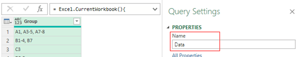
Firstly, we need to load the source data. Select the ‘SplitValueRanges’ table (my name for the input table) with the source data in a single column. To do this, I click on any cell within the table, go to the Data tab in the Ribbon and click on ‘From Table/Range’ within ‘Get & Transform Data’ group.

When the Power Query Editor window appears, I rename the query by entering ‘Data’ into the ‘Name’ field within the Query Settings pane.

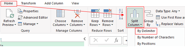
Next, let’s split this Group column.  The first step is to split it by commas to separate multiple values into individual entries.  To do this, select the Group column.  In the Power Query Ribbon, click ‘Split Column’ button within ‘Transform’ group, then click ‘By Delimiter’.

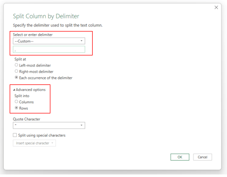
In the ‘Split Column by Delimiter’ dialog, select ‘--Custom--’ and enter “, ” (with a space after the comma).  Expand ‘Advanced options’ and select ‘Rows’, then click ‘OK’.

It should then look like the following screenshot:

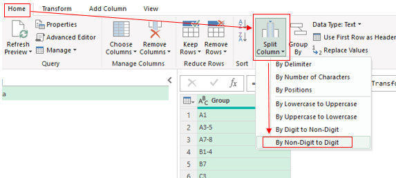
Next, I will continue splitting the Group column, this time separating the alphabetic characters from the numeric values to create a clearer structure.  In the Power Query Ribbon, click ‘Split Column’ button within ‘Transform’ group, then click ‘Non-Digit to Digit’.

To streamline the process and prepare for the next steps, click on the Formula bar and manually rename the column headers by modifying the following formula:

= Table.SplitColumn(#"Split Column by Delimiter", "Group", Splitter.SplitTextByCharacterTransition((c) => not List.Contains({"0".."9"}, c), {"0".."9"}), {"Group.1", "Group.2", "Group.3"})

to
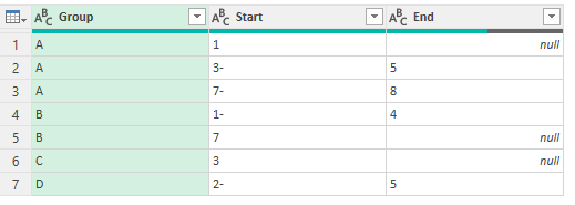
= Table.SplitColumn(#"Split Column by Delimiter", "Group", Splitter.SplitTextByCharacterTransition((c) => not List.Contains({"0".."9"}, c), {"0".."9"}), 
{"Group", "Start", "End"})

It should then look like the following screenshot: 

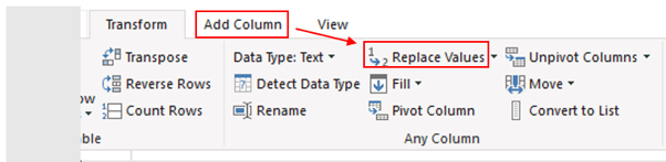
Then, we need to remove the hyphens.  In the Power Query Ribbon, click ‘Replace Values’ button within ‘Any Column’ group.

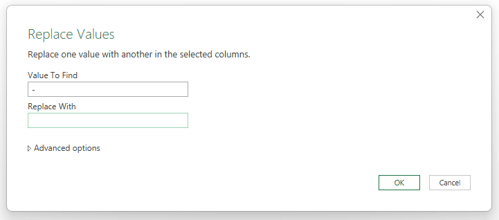
In the dialog box ‘Replace Values’, enter "-" in ‘Value to Find’ and blank in ‘Replace With’.  Click ‘OK’.

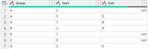
It should then look like the following screenshot:

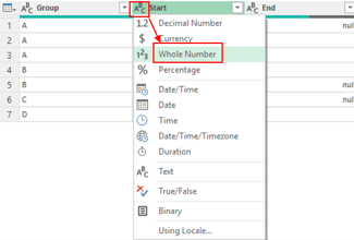
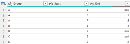
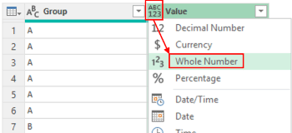
The next step is to change the data type for the Start and End columns to convert the numbers into correct ‘Whole Number’ data type.  To do this, click the icon next to the Start header, select Whole Number, and repeat the same process for the End column.

It should then look like the following screenshot:

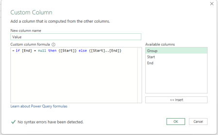
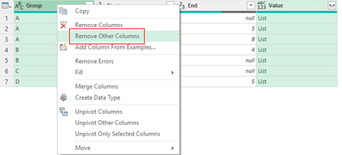
The next step is to generate a list of ranges for each row.  We create a list of values based upon the Start and End columns.  If End is null, it returns only the Start value as a single-item list.  Otherwise, it generates a sequence from Start to End, ensuring both individual values and ranges are correctly captured.  To do this, I add a column by clicking ‘Custom Column’ under ‘Add Column’ Tab.  Please note that Power Query is case sensitive.  In the ‘Custom Column’ dialog, enter the column name as Value and then the formula as below:

= if [End] = null then {[Start]} else {[Start]..[End]}

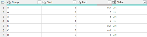
Click ‘OK’ and it should then look like the following screenshot:

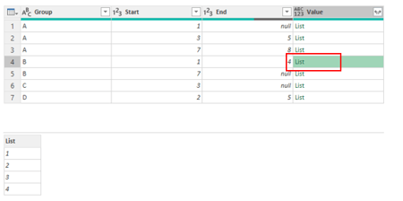
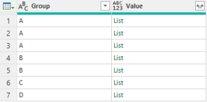
Now the Value has been created, if I click on the blank area next to each ‘List’, I will see the preview of the range list appears at the bottom area like this:

It should then look like the following screenshot:

Then I need to expand Value.  I can expand the Value downward into rows by selecting icon next to Value header and select ‘Expand to New Rows’.

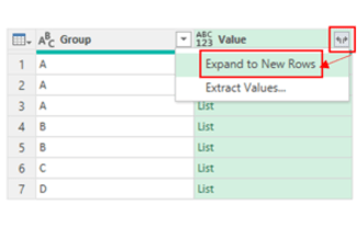
It should then look like the following screenshot:

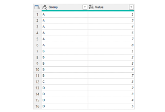
Again, the new Value column has been set to defalt format; I have to change it to the whole number.  To do this, click the icon next to the Value column header, select ‘Whole Number’.

After completing the steps, refresh the queries to ensure all changes are applied, click ‘Close & Load’.

Word to the Wise

Of course, there are many, many ways this could have been achieved.  Hopefully, this approach provides you with some good ideas for future real-life problems…