If you're still working with ranges of data in Excel without the data being stored as an Excel Table (with a capital T), you're potentially making your life much harder than it needs to be. One simple keyboard shortcut can transform how you analyse data, create formulas, and maintain spreadsheets.

Ctrl + T

This shortcut converts a normal range into an Excel Table within seconds.

Many Excel users create complex workarounds for problems that Tables solve automatically. Once you start using them consistently, you'll wonder how you ever managed without them.

What happens when you press Ctrl + T?

Select any dataset and press Ctrl + T. Excel will ask whether your data has headers. Tick the box if you do have headers, click OK, and your range will become an official Excel Table.

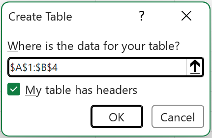
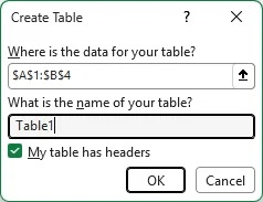
Excitingly, Microsoft has released a long-awaited update (only available to those on Beta Channel at the time of publishing) that will also let you name your table when you create it. Without this, it just gets a default name like “Table1”.

Renaming your Table

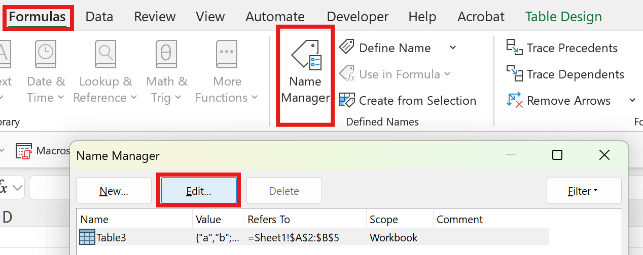
You can rename your table within the Table Design tab that pops up on the ribbon when your active cell is in the Table range. Alternatively, you can go to “Formulas” on the ribbon, then into ‘Name Manager’, selecting your table and clicking “Edit…”.

What’s different with data stored as an Excel Table?

At first glance, you may not notice much difference, but under the hood, Excel has fundamentally changed how it manages your data. It’s now a dynamic object, rather than just a collection of cells.

Your data expands automatically

One of the most common Excel problems occurs when data grows. Without using Excel Tables, if you wanted to add rows to an existing report, there’s a good chance that your new rows will not be included in existing formulas, pivot tables, charts or Power Query connections.

Here’s the magic: with an Excel Table, new rows become part of the Table range automatically. Just add data directly underneath the last row and Excel expands the table for you.

No more manual range updates; no dragging formulas down; and no need to wonder whether your chart is missing the latest transactions. Try it.

Formulas fill themselves in

Let's say you have a "Revenue" column and want to create a "VAT" calculation. In a normal range, you would write the formula in the first row and copy it down hundreds or thousands of times.

In a Table, you enter the formula once and Excel automatically fills the entire column with the same formula. When new rows are added later, the formula appears automatically on the new rows without the need to drag it down.

For large operational spreadsheets, this alone can eliminate lots of user errors. 

Goodbye cell references, hello structured references

Most Excel users become familiar with formulas with basic cell references like: =B2*C2

These formulas work, but they're not particularly easy to read or review, and they’re not very dynamic. In a Table, Excel uses something called structured references: =[@Quantity]*[@Price]

At first this looks strange, but it quickly becomes much easier to understand. Instead of wondering what lives in B2 or C2, you can immediately see that you're multiplying Quantity by Price (in this example, column B header is Quantity and Column C header is Price).

This makes formulas easier to build, audit and maintain. They are also less likely to break. You just have to ensure your column headers are well named.

Pivot Tables become more reliable

Pivot Tables are fantastic, but they often suffer from one annoying problem: every time your source data grows, you need to update your data source.

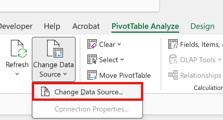
Using an Excel Table solves this instantly. When you build the Pivot Table from an Excel Table rather than a fixed cell range, the Pivot Table data source updates automatically. All you need to do is hit refresh.

Better filtering and sorting

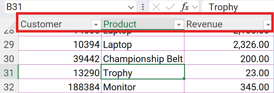
Excel Tables come with built-in filtering and sorting, providing a cleaner experience. 

When you scroll down the workbook, Excel displays the column header names at the top rather than A,B,C, etc. This allows you to filter/sort columns from any row in the table with the drop-down arrow next to the relevant column name. This makes navigation much easier in larger workbooks.

Final thoughts

The best Excel users don't just know more functions, they have built better foundations for working with data.

When you import, copy or create a dataset, press Ctrl + T to convert it from a range to an Excel Table before you start building formulas, charts, etc. It may feel like a small step, but it dramatically improves the reliability of your workbooks.

Just remember this one simple keyboard shortcut: Ctrl + T.

Further reading:

• Principles 8 and 12 of ICAEW's 20 principles for good spreadsheet practice