Excel - escaping from cells - part two

Having opted for practicality, we looked at how to use some of the concepts of database structure to improve the speed and reliability of entering a simple table of expenses data in Excel. This resulted in the creation of three separate Excel Tables: our expenses Table itself, a client Table and a nominal code Table. We finished part one by using Data Validation lists to select our client code and analysis code from the appropriate columns of our Client and Code Tables:

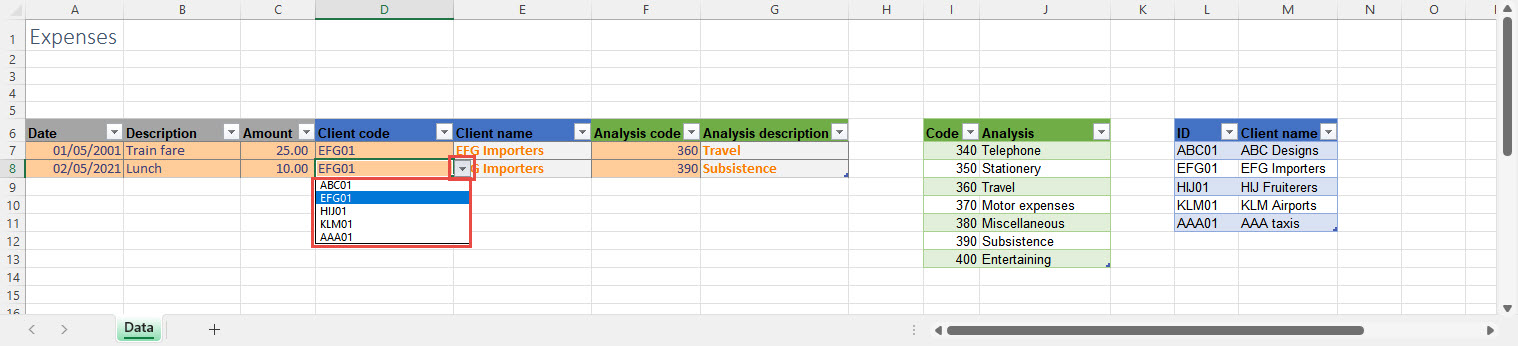
Although using the Data Validation dropdown makes it easier to enter our codes, because the dropdown only shows the single code column from each table, we don't see confirmation that we have selected the correct code. We can address this issue by adding calculated columns to our expenses Table that use lookup formulae to display the Client name and Analysis description. Of course, we could just refer directly to the Client name and Analysis columns without using the Code and ID columns at all, but doing so wouldn't help explain how relational databases work.

One of the most significant recent Excel enhancements has been the long overdue replacement of several of Excel's lookup functions with the new XLOOKUP() function. If your version of Excel doesn't yet include the new function, or if you need to maintain compatibility with older versions, then you can use the exact match form of VLOOKUP():

=VLOOKUP([@[Client code]],Client,2,FALSE)

With VLOOKUP() we need to specify 4 arguments:

• The value to be found in the client Table. In this case the value in the Client code column, current row of the expenses Table;
• The Table that contains the value we want to find in the first column and the value we want to return in another column. In this case our Client Table;
• The number of the column that contains the value to return. In this case column 2;
• The type of match to perform. In this case FALSE for an exact match. Forgetting to specify this fourth argument will lead to VLOOKUP() performing an approximate match and returning an apparently unpredictable value.

The XLOOKUP() equivalent is:

=XLOOKUP([@[Client code]],Client[ID],Client[Client name],"No such client")

Again, we have four arguments:

• The value to be found is the same as for VLOOKUP() above;
• The list of values that contains the value to find. In this case just the ID column of the Client Table;
• The list of values from which to return the required value. In this case just the Client name column of the Client Table;
• The fourth argument this time is the value to return if no match is found. XLOOKUP() defaults to using an exact match so there is no need to specify this.

If we needed to ensure that the VLOOKUP() formula returned anything but a #N/A error when there was no match we would need to also use an information function such as IFNA():

=IFNA(VLOOKUP([@[Client code]],Client,2,FALSE),”No such client”)

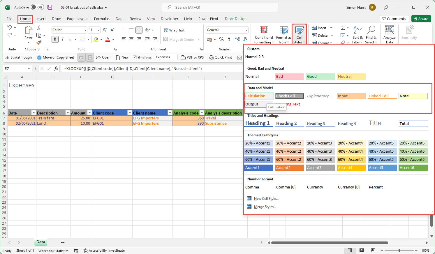
As we mentioned in the previous episode, because we have created our Expenses table as an actual Excel Table, our XLOOKUP() formulae in columns E and G will automatically be copied down to new rows as they are added. The inclusion of calculated columns in our data entry table is not without its issues. Going back to the ICAEW 20 Principles, Principle 10 states that you should "Separate and clearly identify inputs, workings and outputs". Obviously, in this case we need our lookup columns to be in the same Table as our data columns, rather than being separate, but we can at least comply with the 'clearly identify' aspect of the principle by using cell formatting to distinguish data entry cells that we want our user to enter information into, from calculation cells that we don't want them to change. We have used the Calculation and Input styles from the 'Data and Model' category of Cell Styles to apply our formats:

To recap, in part 1 we pointed out the disadvantages of duplication in a data entry table, including the contribution that duplication makes to the likelihood of errors occurring. By using Data Validation lists and lookup formulae, we have ensured that we only need to type in our Analysis description and Client name once in each of their respective Tables, yet we can still display the full information in our Expenses data entry Table.

Our approach is far from perfect. As useful as Data Validation is, it's not necessarily a completely reliable way to prevent users entering incorrect data. Also, a longstanding bug in Excel prevents us from applying Principle 20: "Protect parts of the workbook that are not supposed to be changed by users". Formula cells can be locked, and a worksheet protected, to prevent users changing formulae, inadvertently or otherwise. However, the Excel bug means that protecting a worksheet disables the ability to add rows to any Tables on that worksheet, rendering locking and protection unusable on most worksheets that incorporate Tables.

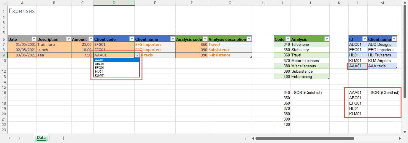
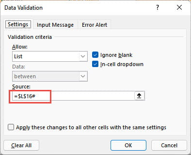
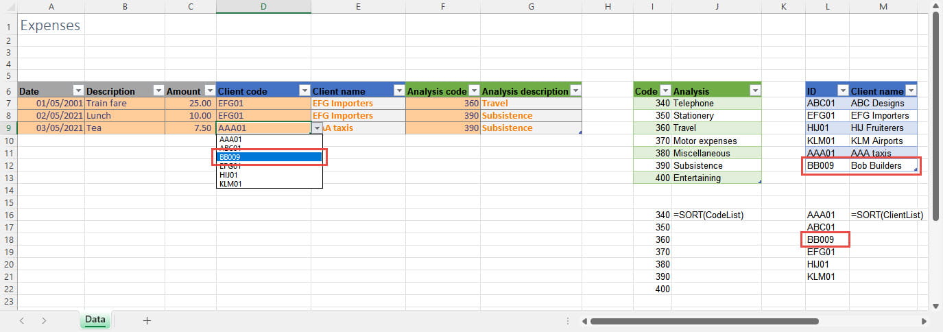
There is another, practical issue. Our dropdown lists work well enough with up to a dozen or so entries in our subsidiary Tables, but many more items than this would make the lists cumbersome to navigate. The problem is compounded by the potential lack of sorting in our subsidiary Tables. By default, our dropdown lists will just be displayed in the order that the Table entries were made. Following the introduction of Dynamic Arrays in Excel, the sort problem is relatively easy to address. We can use the Dynamic Array SORT() function to sort our lists. The resulting formula will expand dynamically as any new rows are added. Just for demonstration, we have entered our SORT() formulae in single cells just below the corresponding columns. We have also followed the advice in part 1 to apply Range Names to our lookup columns, using CodeList for our Code column and ClientList for our client ID column, so we can just enter SORT(CodeList) and SORT(ClientList). Because we are referring to single columns, we don't need to use any of the optional SORT() arguments. Our Dynamic Array SORT() formula 'spills' down to as many cells as are required to include all the entries from the source range:

Having created our sorted lists, we can refer to them dynamically using the cell into which they are typed, followed by the # character which expands the reference to the entire 'spilled' range of cells:

We can see the automation flow through here as we add a new row to our Clients Table:

In conclusion, although we can improve certain aspects of entering data into an Excel worksheet by understanding how to split data into separate tables, we are still left with reliability and usability disadvantages that using a database application would overcome. However, understanding the basics of how to split data into multiple tables and then recombine them using lookup formulae provides a good introduction to working with external sources of data using indispensable tools like Power Query for example.