How to review a spreadsheet: Part 6 - other useful functions

Inspecting the workbook

Tucked away under the File menu is a diagnostic tool where you can select up to 22 attributes to be reviewed and the findings generated.

Select File and the from the list down the left of the screen select Info. The second block down is Inspect the Workbook. Click on the square icon ‘Check for issues’. The first option is ‘Inspect Document’. Initially a warning emerges asking you to make sure the document is saved before progressing. It may be best to save a separate version on which you apply this feature.

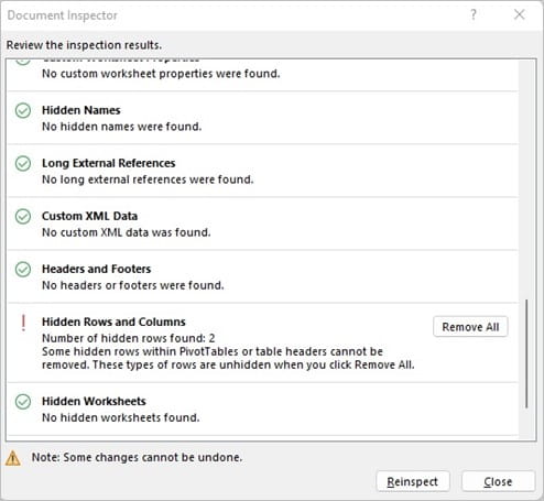
You can now select the attributes you would like examined and press inspect. In response the details of any issues are then listed for validation or removal. The details reported are not hugely explicit. For example, in the screen shot below it states that it found two hidden rows, but it does not tell which they are. You must go and find them out for yourself.

Hidden attributes

It is possible to hide spreadsheet details whether they be Worksheets, rows/columns, text or numbers. All can be revealed as follows:

WORKSHEETS

To reveal Worksheets that may be hidden right click any tab at the bottom of the Worksheet and select Unhide and a dialog box will list the available hidden sheets.

However, in Visual Basic there is a third status called ‘Very Hidden’ that can only be selected and revealed using the VB Editor. To identify whether there are any ‘Very Hidden’ Worksheets type the function =INFO(“NUMFILE”) into any cell and the result displayed is the number of Worksheets in the Workbook. If the total does not equal the number that is visible, then you know there are additional hidden Worksheets to be revealed.

ROWS/COLUMNS

To reveal any rows or columns that may be hidden start by pressing CTRL and A (select all) this will highlight the whole Worksheet. Then right click on any column and select Unhide. Similarity, right click on any Row header and also select Unhide.

TEXT

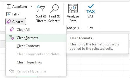
To reveal text that might be hidden press CTRL and A (Select all) and temporarily clear all formatting by going to the Editing section of the Home Ribbon. Under the Clear option select Clear Formats. This will remove all formatting including white font on a white background.

NUMBERS

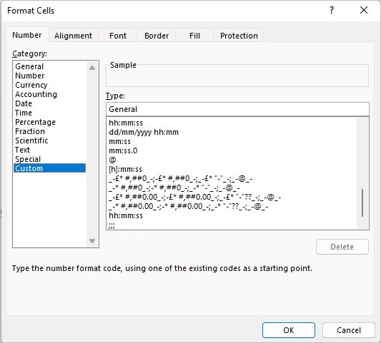
Another way that numbers may have been hidden is by using a Custom Format that will display as blank. In the Number Section of Home Ribbon click on the small black arrow in the bottom right corner to open the Format Cells Dialog Box at the Number Tab. Using the Custom Format of ;;; will hide all numbers using this Format. First scroll down the options available to see if that format has been set up (as shown below). Any numbers where it has been applied can be revealed by the Clear Format option explained above. Alternatively delete the format from the list and all numbers which are using it will revert to the standard display format (highlight the style and press the Delete button at the bottom of the dialog box).

Recalculation

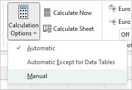
A spreadsheet is normally set up with automatic recalculation, such that every time the Enter key is pressed the spreadsheet will automatically recalculate. However, it is possible to turn this to Manual recalculate so that calculation only occurs when the F9 key is pressed. The typical reason it might be changed is for a large spreadsheet with multiple Look ups and it takes more than a moment to compete the recalculation.

The danger of the manual mode is that data can be updated and then the results used for decision making with a recalculation having taken place.

There is function that can be typed into any cell that will reveal the recalculation status =INFO(“RECALC”) and it will reveal the answer Manual or Automatic.

To switch between the two modes go to Formulas Ribbon and the Calculation section.

Series concludes

I hope these blogs have been helpful to you in learning how to apply the principles covered in the ICAEW publication on ‘How to Review a Spreadsheet’.

The blogs are written by John Tennent, a Chartered Accountant and Managing Director of Corporate Edge Ltd. He is a member if the ICAEW Excel Community Advisory Committee. He is the Author of ‘The Economist Guide to Business Modelling’ and both builds models for clients as well as runs training courses to help people build their own models. He can be contacted on john-tennent@corporateedge.co.uk