Excel at Christmas

Introduction

For Christmas 2023 we included a community post to create a spreadsheet Christmas tree with randomly flashing lights and for 2024 we calculated how many gifts were given across the 12 days of Christmas. After a Christmas off, this year we turn our attention to an Advent calendar.

The aim is to create a worksheet with 25 Advent calendar doors that automatically open a day at a time from December 1 to December 25.

Behind the doors

To start with, we need some festive pictures to place behind each of our 25 doors. We want each picture to be placed in its own cell so that we can retrieve each one individually using the equivalent of a cell reference. We can use a relatively recent option to do this. From the Insert Ribbon tab, Illustrations group, the Pictures dropdown includes a Place in Cell sub-option. From this we can choose from a variety of picture sources. We will use Stock Images:

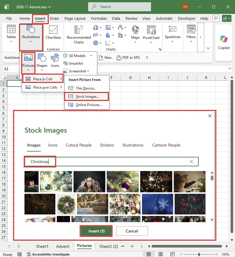
We could search the stock images gallery for ‘Christmas’ pictures and then insert 25 different pictures individually. However, there is a quicker way. Having selected cell A1 we can search for ‘Christmas images and then select 25 in one go, before inserting them:

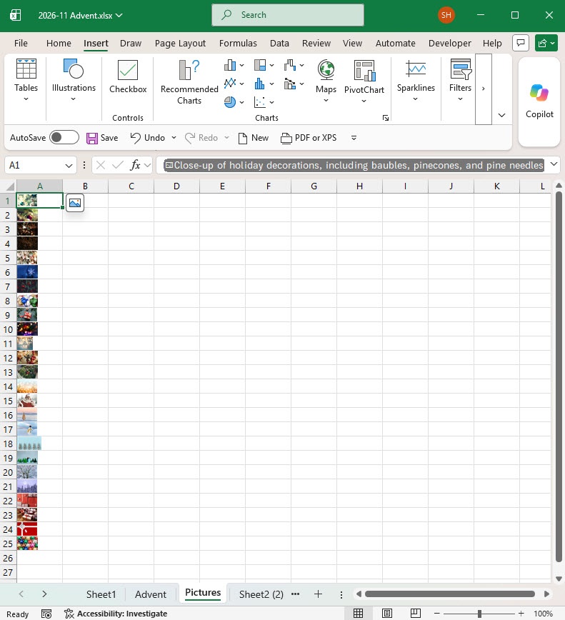
In order to make our pictures easier to access and our formulas easier to understand, we are going to select the cell range A1:A25 and use the name box just to the left of the formula bar to give the range the name ‘Pictures’.

We will then follow the same steps to find pictures of doors and paste a single, suitable picture in cell C1. We will allocate the range name ‘Doors’ to this single cell in the same way that we named our range as ‘Pictures’.

Our Advent calendar

On a separate worksheet, we are going to use the block of 25 cells, A1 to E5 to hold our pictures. We can use the INDEX() function to choose a single picture. For example, entering in cell A1 the formula:

=INDEX(Pictures,5)

will display the fifth cell in our Pictures range.

However, we do not want to create a long, thin Advent calendar 25 columns wide or 25 rows deep. To create our neat 5x5 block we will create an array of the numbers 1 to 25 in a block using the SEQUENCE() array function:

=SEQUENCE(5,5)

We want to allocate our pictures sequentially to the cells in the block using the row and column positions of our 25 cells:

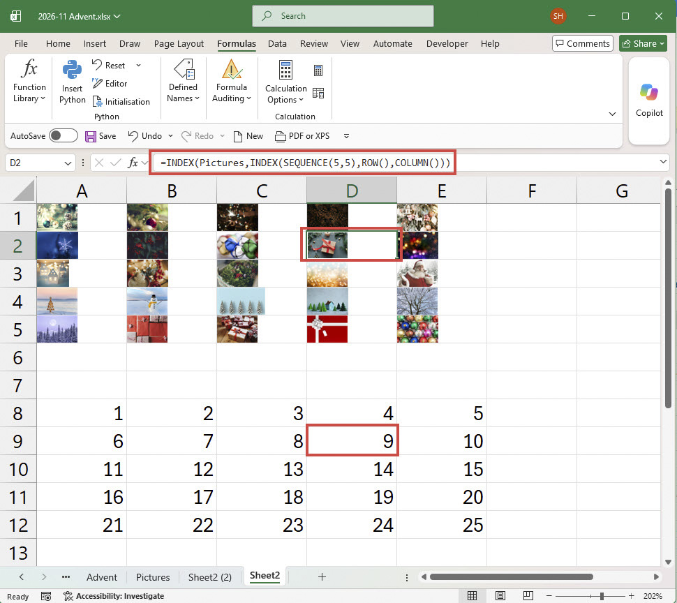
=INDEX(Pictures,INDEX(SEQUENCE(5,5),ROW(),COLUMN()))

The second INDEX() function uses the row and column position of each cell to find the correct number in our 5x5 block. For example, cell D4 finds the ninth value in our block, the value 9. The overall INDEX() function uses this value to retrieve the 9th cell from our Pictures Range:

As an alternative approach, we could do the same thing, and avoid the use of the SEQUENCE() function, by arranging our pictures in a 5x5 block in the first place.

Automatic doors

Finally, we will enable our doors to open automatically from December 1st onwards. We will do this by adding a formula that counts the number of days from today until the date of December 25th 2026, which we have entered in cell G1

=G1-TODAY()

We will name this cell:

AdventDays

We can then enter the following formula in our 25 Advent Calendar cells:

=IF(25-AdventDays>=INDEX(SEQUENCE(5,5),ROW(),COLUMN()),INDEX
(Pictures,INDEX(SEQUENCE(5,5),ROW(),COLUMN())),Doors)

The IF() function compares the index number calculated from the row and column position of each cell with the number of days between today’s date and 25th December, subtracted from the total number of cells: 25. On December 1st there will be 24 days difference and 25-24=1 so only the first cell in the block will display one of the Pictures range and the other 24 will display the Doors picture.

We could use the LET() function to simplify our formula slightly:

=LET(CalendarDay,INDEX(SEQUENCE(5,5),ROW(),COLUMN()),IF(25-AdventDays>=CalendarDay,INDEX(Pictures,CalendarDay),Doors))

As it’s mid-November at the time of writing, in order to demonstrate what will happen in December, we have temporarily replaced the use of the TODAY() function in the AdventDays cell to use the value in cell G2 instead:

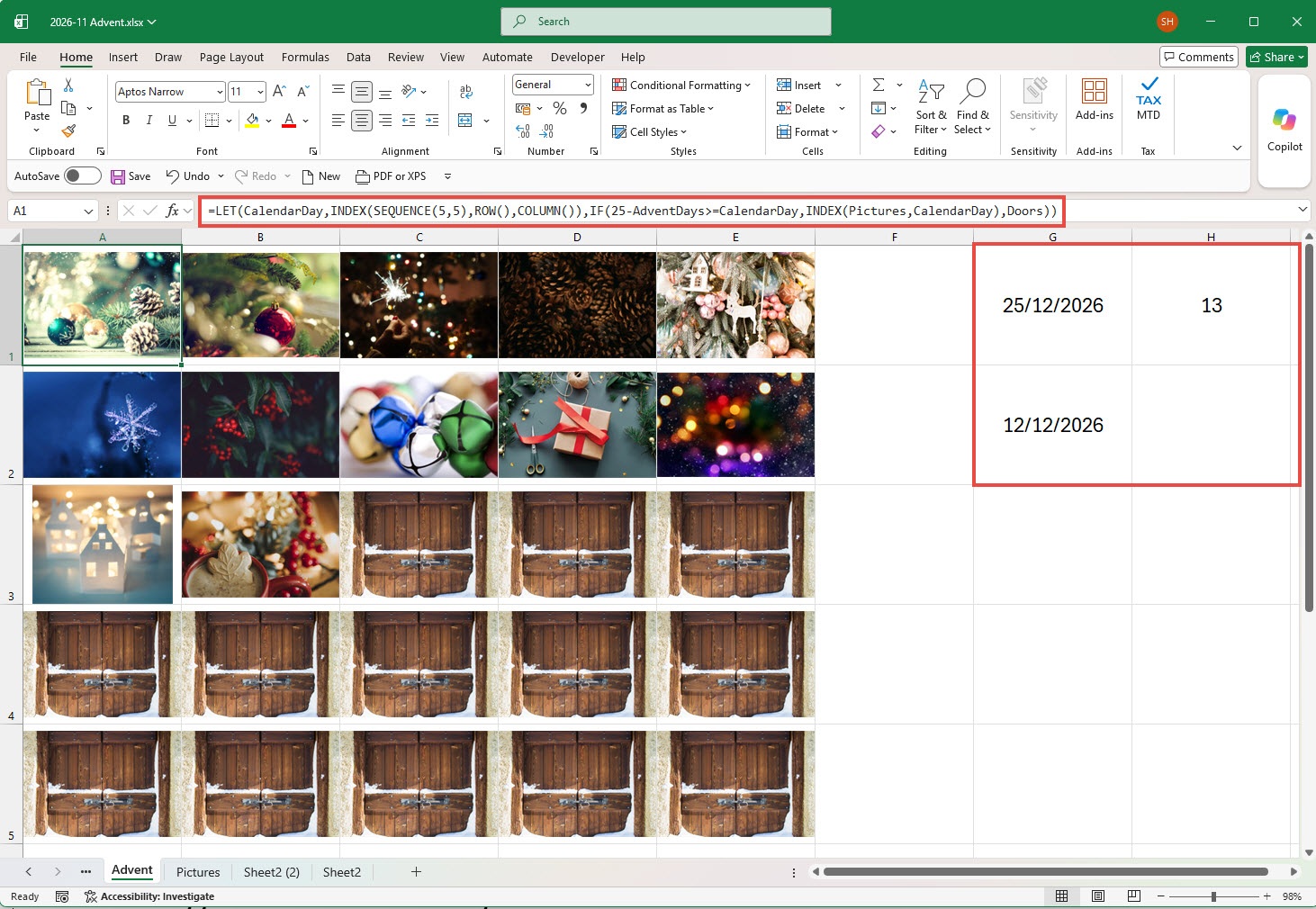
Our Advent calendar will update for today’s date when using the TODAY() function whenever there is a recalculation.

Additional resources

The Power BI based ICAEW Excel archive portal includes several seasonal articles. Select the ‘Christmas Specials’ series/topic to see a list:

The 'Open in full-screen mode' icon in the bottom right-hand corner of the embedded report should show the contents at a more readable size with the Escape key returning you to the post.