Animated Excel Christmas Tree

Such was the response to our pre-Christmas post on using Conditional Formatting and Dynamic Arrays to create an animated Christmas tree, that we are starting the New Year with a follow up post covering possible ways to address the additional challenges the article included.

Just to recap, the previous article looked at the creation of a Christmas tree in an Excel worksheet animated with coloured lights. After experimenting with a range of ‘normal’ Excel formulas and Conditional Formatting, we went on to use a Dynamic Array to create our animated Christmas tree using a single formula. This was based on the the MAKEARRAY() function which uses a LAMBDA() function as one of its arguments:

Our suggestion for filling up spare time over the Christmas period was to add a pot or stand for the Christmas tree and make the height and width of the trunk changeable based on cell values. Our stretch target was to add a coloured background with random snowflakes.

We’ll add a couple of values to the existing list of variables in our workbook to hold a trunk height value and a width value and we’ll allocate Range Names to these two values: TWidth and THeight. We’ll then change the Conditional Format that creates our Christmas tree trunk to use these two variables rather than fixed values:

=AND(ABS(COLUMN()-Width)<TWidth,ROW()>Width,ROW()<Width*Theight)

In the previous article we had used a value of 3 for the trunk width. Because our formula draws the drunk either side of the middle position, the actual width in columns will be twice the value we enter as our TWidth variable.

Later, we are going to add a coloured background to our picture. This will be set to fill a square with sides twice our overall width value. We don’t want our trunk to extend below the bottom of our background, so our THeight value needs to be set to a decimal value between 1 (no trunk) and 2 (trunk the same height as the tree itself.)

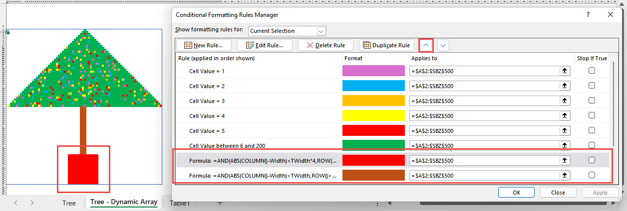
We will duplicate our trunk Conditional Format in the Conditional Formatting Rules Manager and change it to create a pot for our tree to stand in. For simplicity, we have just set it to be four times as wide as our trunk. We need the pot to be positioned at the bottom of our trunk, so we add an additional condition to our AND() function to only use our pot Conditional Format for columns in the ‘width’ area, and for row numbers that are less than our calculated trunk height, and more than 80% of the trunk height. So, the pot should be four times the width of the trunk and cover 20% of the full tree height from the bottom of the trunk upwards. We have chosen red as the colour of our pot.

=AND(ABS(COLUMN()-Width)<TWidth*4,ROW()>Width,ROW()<(Width*THeight),ROW()>(Width*THeight*0.8))

We can see that we have a small problem. Although our pot appears, the trunk shows through it. This highlights one of the less intuitive aspects of how Conditional Formatting works with multiple rules. You might think that the rules are applied in the order in which they are shown. However, if this was the case, the red conditional format would overwrite the brown conditional format. In fact, the order of the rules is only relevant when one or more rules are set to ‘Stop if True’, or where multiple rules evaluate as TRUE, as is the case with our trunk and pot rules. Where multiple rules are true, the order determines which will be applied, with the rule higher up in the list taking priority. If we select our pot Conditional Format and use the up button to move it above our trunk Conditional Format, it will take priority and our trunk will not show:

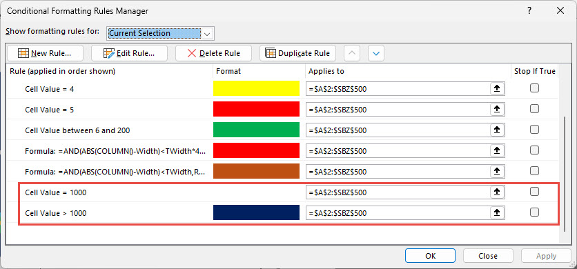
We have used two more Conditional Formats to set the background colour and falling snow. We have also changed the FALSE argument of our array formula from “” to create a blank cell, to adding a random number between 1000 and 1020:

=MAKEARRAY((Width-1)*2,(Width-1)*2,LAMBDA(treerow,treecolumn,IF
(AND(treerow<Width,treecolumn>Width-treerow,treecolumn<Width+treerow),RANDBETWEEN
(1,Lights),RANDBETWEEN(1000,1020))))

Our background colour will we applied to all the cells with a value over 1000 and our snow colour will be applied to all cells with a value of exactly 1000, so approximately 5% of our background cells will be snowflakes. Increasing the second RANDBETWEEN() value from 1020 will decrease the percentage of snowflakes. Just like our Christmas tree lights, the position of the snowflakes will change randomly each time our workbook is recalculated:

You can explore any of the various techniques we have covered here in the ICAEW Excel Community archive.