Handling missing columns in Power Query

One of the most common causes of Power Query errors is columns that no longer exist. It is common for inputs that have an unknown number of columns.

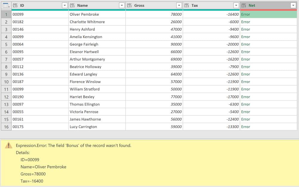
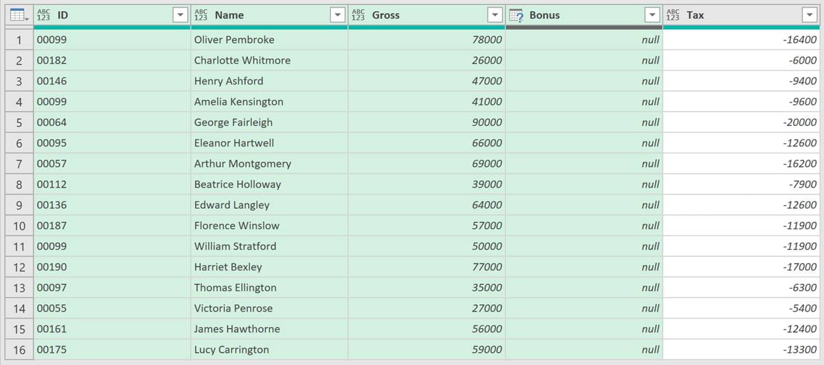
For example, a payroll report might include columns for Gross, Bonus, Tax, etc. But if there is no bonus for a specific month, the Bonus column is often excluded.

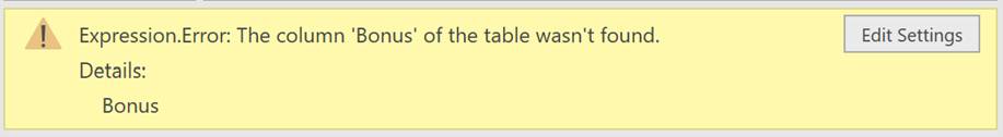
If we reference the missing column anywhere in our query, we get a familiar error.

In this post, we will look at some common solutions to help us avoid this and get the result we need.

Example scenario

The example we are using is simple.

We simply want to add the Gross, Bonus and Tax values to calculate the Net pay.

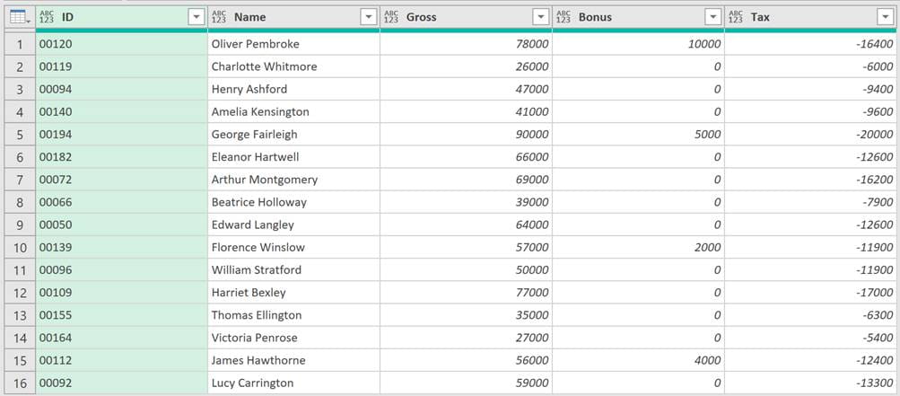
The data starts as follows:

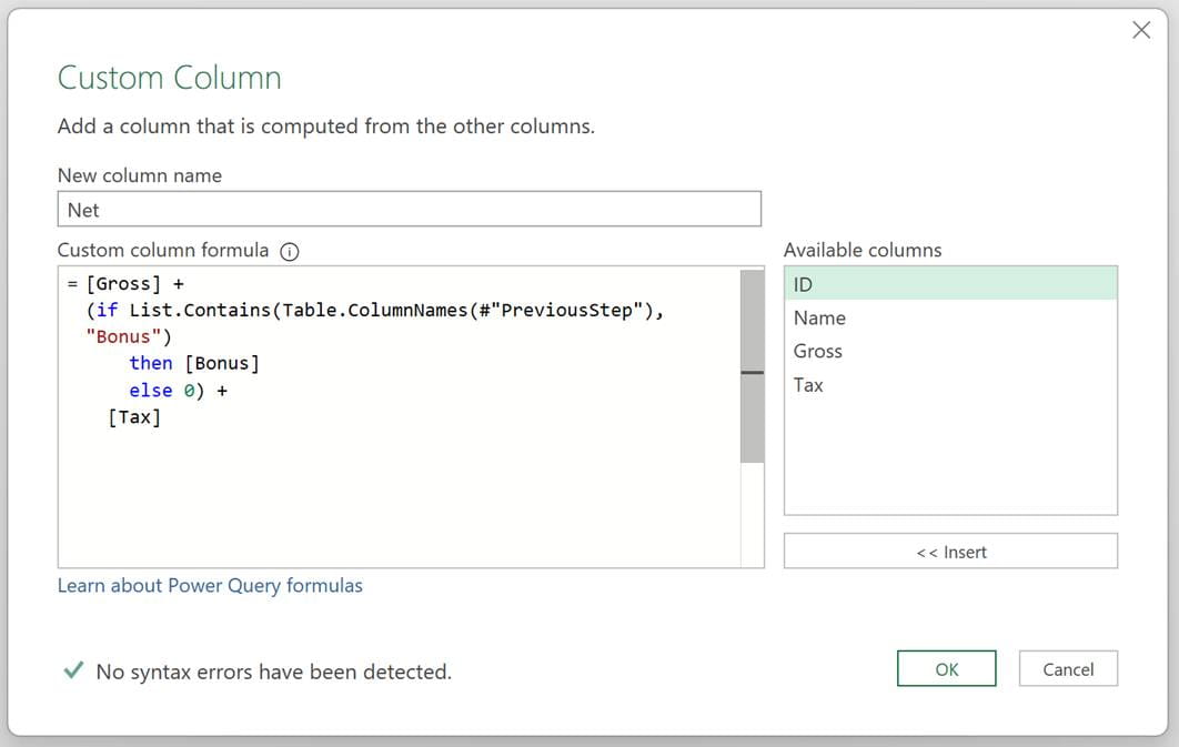
To add the Net pay calculation in Power Query we click Add Column > Custom Column in the ribbon, and enter the following:

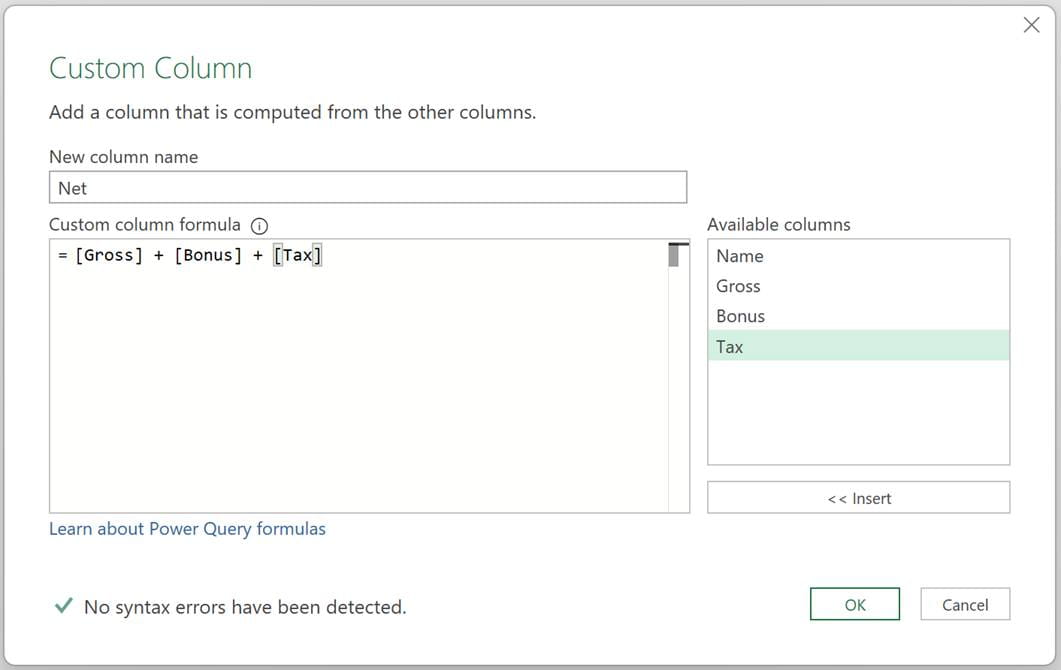
The tax value is negative, so the formula is:

= [Gross] + [Bonus] + [Tax]

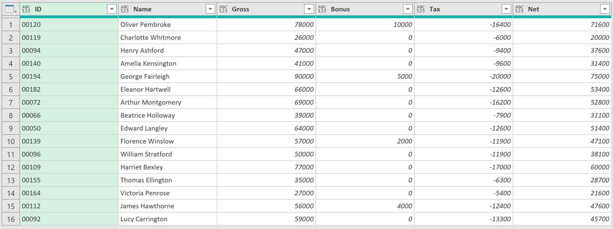
This adds the Net column to the table.

However, when we update the data for the following month, the Bonus column could be missing. As a result, we get an error.

Now, let’s work through some solutions to resolve this.

Check if a column exists

The most explicit approach is to check if a column exists before referencing it.

The following M code retrieves the list of column names from the previous step and checks whether Bonus exists in that list.

List.Contains(Table.ColumnNames(#"Previous Step"),"Bonus")

This formula returns true if Bonus exists, or false if not. Therefore, we could use that inside an if statement.

The formula would become:

= [Gross] +
(if List.Contains(Table.ColumnNames(#"Previous Step"),"Bonus")
then [Bonus] else 0) +
[Tax]

The formula checks if the Bonus column exists. If it does, the Bonus value is included in the calculation; if not, the calculation uses 0.

This approach uses an if statement to check whether a column exists before referencing it.

Provide an alternative if an error occurs

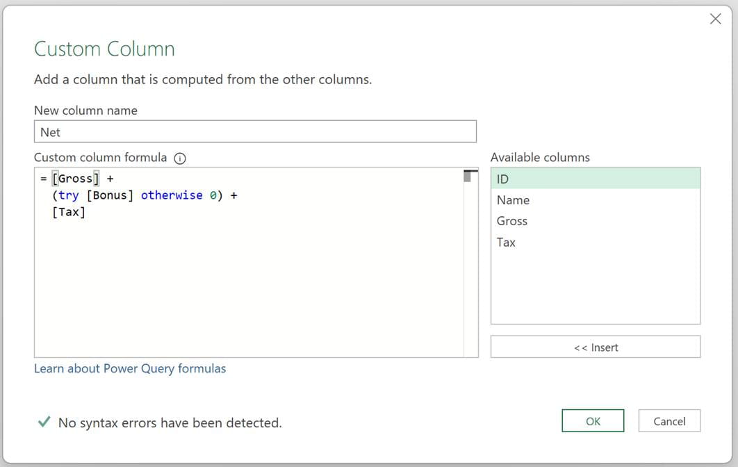
A related option is to allow the calculation to occur but provide an alternative if it creates an error.

The formula could become:

= [Gross] +
(try [Bonus] otherwise 0) +
[Tax]

The try keyword executes the code, and the otherwise keyword executes only if an error occurs.

So, if the Bonus column does not exist, 0 is returned.

This provides the same results as the previous example, but with slightly shorter syntax.

Optional field access and coalesce operators

Power Query has two special operators:

• ? – Optional field access operator – returns null if a field does not exist
• ?? – Coalesce operator – returns the first non-null value

We can use these two operators together to get an equivalent result to the methods above.

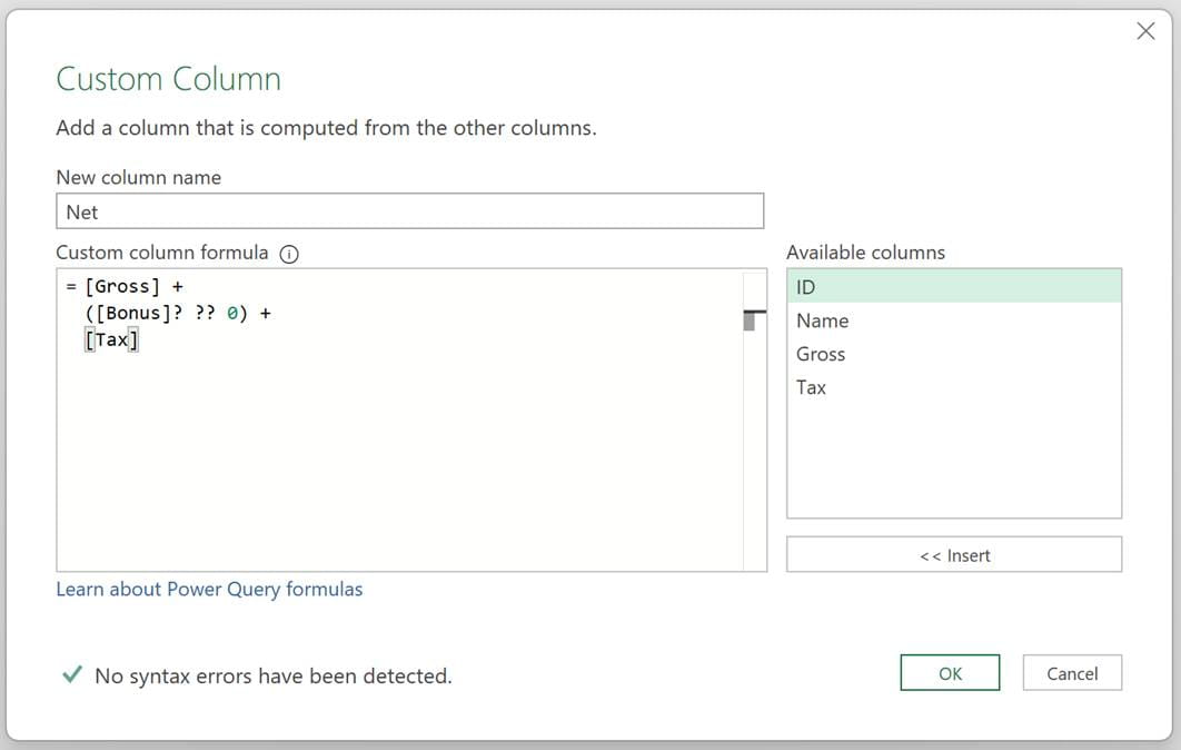
We can enter this logic into the Custom Column dialog box.

The formula is:

= [Gross] +
([Bonus]? ?? 0) +
[Tax]

[Bonus]? returns the value from the Bonus column, or null if the column does not exist.

Adding ?? 0 returns the first non-null value. Therefore, as a whole section, [Bonus]? ?? 0 returns the bonus if it exists, or 0 if it does not.

It takes a bit of thought to understand how the null values are handled in this scenario. But it returns the same result as the previous methods and has even shorter syntax.

MissingField enumerator

If there were a lot of columns to check, the solutions above would become quite cumbersome.

So, let’s take a look at a different approach entirely. We will force the columns to exist before we use them. Apply the following steps before the Custom Column.

Start by selecting all the columns in the Table. Click Home > Choose Columns from the ribbon.

When the Choose Columns dialog box appears, ensure all the column names are selected. Click OK.

The formula bar will show something like the following.

= Table.SelectColumns(#"Previous Step",{"ID", "Name", "Gross", "Tax"})

There are two changes we want to make:

1. In the list of column names, include all the columns.
2. Add the end of the formula, enter the MissingField.UseNull option.

The formula becomes:

= Table.SelectColumns(#"Previous Step",{"ID", "Name", "Gross", "Bonus",
"Tax"}, MissingField.UseNull) 

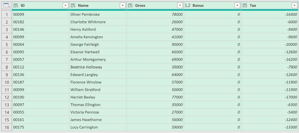
Any missing columns are added with null values.

Unfortunately, we’re not quite finished. Null is not recognized as a number, so our Custom Column will not calculate correctly. 

We need to convert the nulls to 0s. Let’s add another step.

Select all the columns in the Table. In the ribbon, click Transform > Replace Values.

In the Replace Values dialog box, enter the following:

• Value To Find: null
• Replace With: 0
• Click OK

The code in the formula bar will look like the following:

= Table.ReplaceValue(#"Removed Other
Columns",null,0,Replacer.ReplaceValue,{"ID", "Name", "Gross", "Bonus",
"Tax"})

The table column names are hardcoded into this formula. To ensure this includes any new columns, we are going to the list:

{"ID", "Name", "Gross", "Bonus", "Tax"}

With this:

Table.ColumnNames(#"Removed Other Columns")

Note: Removed Other Columns is the name of the prior step.

The final formula becomes:

= Table.ReplaceValue(#"Removed Other
Columns",null,0,Replacer.ReplaceValue,Table.ColumnNames(#"Removed Other
Columns"))

We now have all the columns we need with values.

NOTE: This method will replace null values in all columns, so you will need to separately handle the null values inside non-numeric columns before applying this.

The Custom Column calculation will now be straightforward because the required columns will always exist.

Add all columns except…

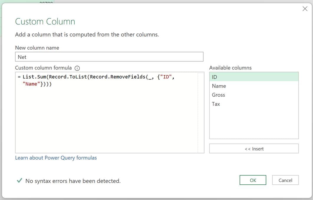
There is one final method we will look at. We use this when we want to remove the fields from a given list and sum everything that remains.

The formula is:

= List.Sum(Record.ToList(Record.RemoveFields(_, {"ID", "Name"})))

Let’s look at this formula by working from the inside out.

• Record.RemoveFields(_, {"ID", "Name"}): Removes the ID and Name fields, leaving the remaining fields.
• Record.ToList(…): Each row is converted into a list of values.
• List.Sum(…): Sums the values in the list.

It doesn’t matter how many columns appear. Provided they are not called ID or Name they will be included within the calculation.

This method works where all the columns should be included in the result, no matter what they are.

Conclusion

In this article, we have seen 5 different methods for handling missing columns. It is certainly not an exhaustive list. Other scenarios with different nuances will require slightly different approaches. The key is to understand your data and create an appropriate solution.

So, if you ever have a missing column scenario in the future, don’t think, “Power Query won’t work for this”. Instead, you should think, “There must be a way for Power Query to do this”… and usually, there is.