Smoothing Capex

To recap, perhaps the easiest way to think of it is as follows:

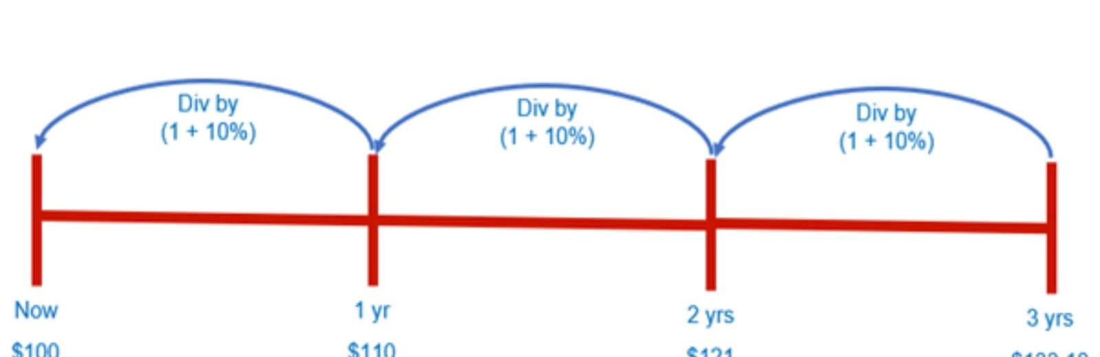
• Let’s assume inflation is running at 10% (and we will assume this is after tax as we all earn our wages after tax and increases in spending affect this after-tax wage)
• Something that costs $100 this year will cost 10% more next year, i.e. $110
• Something that costs $110 next year will cost 10% more the year after, i.e. $121
• Something that costs $121 in that year will cost 10% more the following year, i.e. $133.10
• However, they are all worth the equivalent of $100 now (as we “discount” these future values back to their present values).

Note that all of these valuations are for a point of time not a period.  This is a common mistake in modelling.  We have to understand when we assume the cash flows will occur.  The three most common assumptions are at the start, the middle or the end of the period in question.  This assumption will obviously vary the overall valuation as a consequence.

Valuations include both cash inflows and cash outflows.  Adding up all these positive and negative present values, provides a netted off total: the Net Present Value (NPV).  The aim is to generate a positive return (a positive NPV) for a given rate of discounting, known as the discount rate.

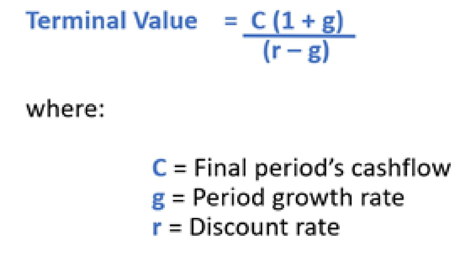
Often, we assume a project or a business will go on “forever” (in perpetuity).  Well, I don’t have enough columns for that, so once cashflows start to settle down into more predictable growth patterns we will often calculate a final figure, known as the terminal value, which is based upon the final period of a cash flow to represent the value of future cash flows after this point in time.  It is typically calculated in perpetuity (as I mentioned above) and uses the formula:

Now that’s fine if the cash flows have indeed settled down – but that’s not always the case.  The most significant figure that often refuses to grow smoothly is capital expenditure.  That’s because we often have to acquire large ticket items on a cycle (e.g. economic life of four years for vehicles, 10 years for plant and machinery) and taking any one year’s figure will not adequately represent upcoming costs.  Given the terminal value is often a material figure in the NPV, getting capital expenditure right is essential.

There are ways to smooth out the capex to make it predictable so that we may have a representative number for the terminal value:

• Some simply average the expenditure over time.  Depending upon how this is done, this may not consider inflation, nominal / real considerations or other time value of money issues
• Some use depreciation as a proxy.  This is a common approach, especially when calculating tax, but it depends upon whether depreciation is a good approximation to the average (it may not be if an item is still in use that has been fully depreciated) or what method of depreciation is used (e.g. straight line or declining balance)
• More sophisticated methods using annual equivalent discount factors and segregating the capital expenditure by useful economic lives.

Well, guess what?  I am not going to do any of those.  I am going to demonstrate another method that will also hold up to scrutiny as I will replace a capital expenditure profile for another “smoothed” one over the same time period that will have an identical net present value. There are issues with this approach (e.g. if the capex profile provided is not representative), but many of the problems associated with this technique could be levelled at any or all of the methods out there.

To demonstrate this approach, I am going to use the attached Excel file as an illustration. Consider the following:

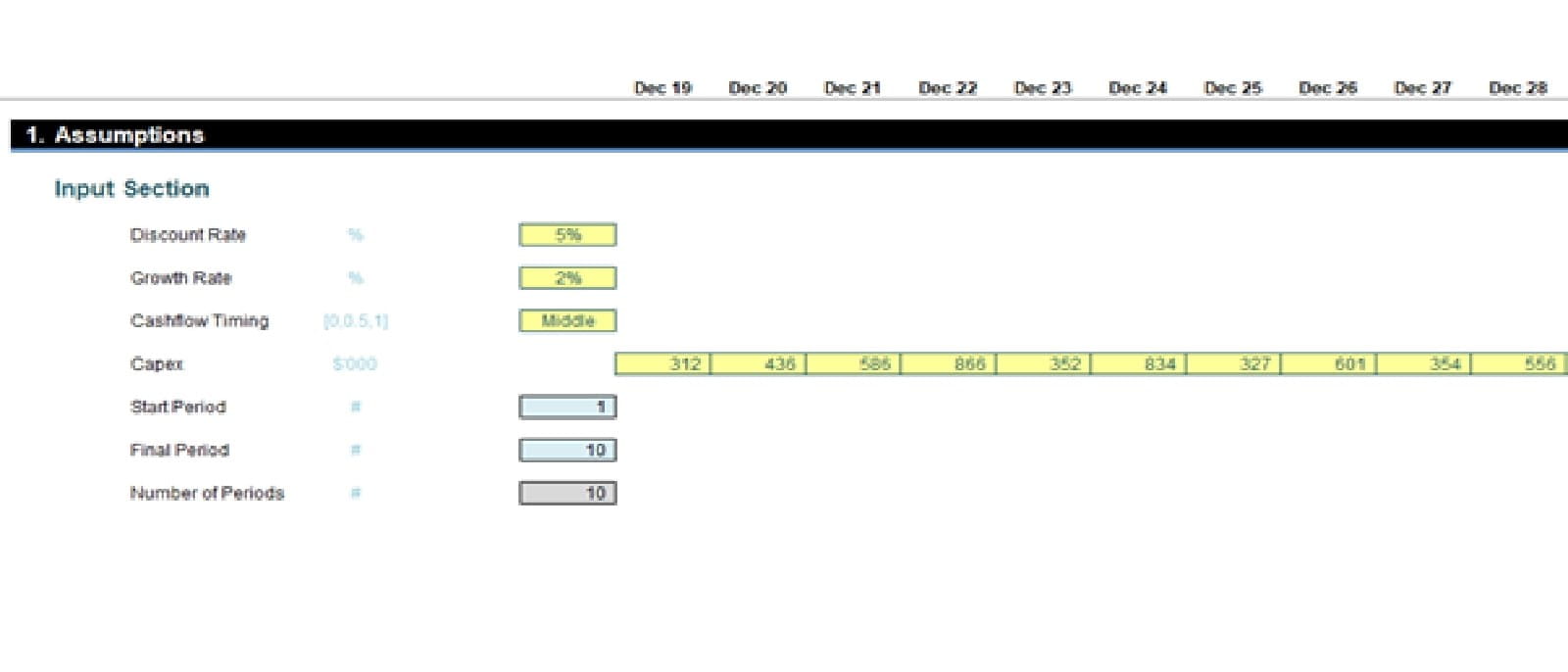
Here, I consider 10 full years (i.e. no “stub” beginning or end periods) with percentages quoted per annum.  The same technique employed here may be used for full months, quarters or half years too – provided the percentages are calculated accordingly.  Remember, there will be no terminal value in our calculations as we are doing this in order to calculate what is required for the terminal value.

It’s also worth noting in the data (above):

• The nature of the discount rate is frequently debated.  Some will argue that this must be the rate implicit in the equivalent leasing of the expenditure, others the inflation rate in the item and the other the discount rate of the larger valuation.  I will leave that to better minds to argue that.  That’s the beauty of being a modeller – it’s just an input figure to me!
• Growth rate is much more self-explanatory.  The idea is to replace the profile pictured with a base “smoothed” capex figure that may then be grown at this growth rate each period, which will produce the same Net Present Value as the original cashflows
• The cashflow timing has three alternatives: cashflows occur at the start of the period, the middle or the end.  This has an impact on the calculated discounted factors
• The capex numbers are the original outflows.  The example file allows you to put a profile in for up to 30 periods, even allowing for an initial delay.

The Start_Period is given by the formula

=IFERROR(MATCH(TRUE,INDEX(Capex_Profile<>0,),0),1)

This formula is the opposite of the usual INDEX(MATCH) syntax.  The calculation INDEX(Capex_Profile<>0,) creates a virtual vector (list) of TRUE and FALSE depending upon whether each item in the range Capex_Profile is blank / zero (FALSE) or not (TRUE). 

MATCH(TRUE,INDEX(Capex_Profile<>0,),0) simply returns the first non-zero / non-blank occurrence, and IFERROR is used just in case there are no values.

The Final_Period is given by the array formula (entered using CTRL + SHIFT + ENTER)

{=MAX(IF(Capex_Profile>0,LU_Counter))}

and returns the largest value in LU_Counter where LU_Counter is the period number (hidden in the graphic above), i.e. it gives the final period where the expenditure is greater than zero (this could be replaced by not equal to zero, for example).

The Number_of_Periods is then easy. It is simply equal to

=Final_Period-Start_Period+1

Do remember to add the one (it’s a common mistake otherwise)!

In order to calculate a Net Present Value, I am going to need some discount rates: three in fact.

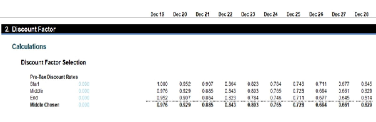
The formulae in the attached Excel file are more complex as they allow for delays and the number of periods to be flexed, but essentially the formulae simplify to

=1/(1 + Discount_Rate)^(Period_No – 1 + Adjustment Factor)

Where the Adjustment_Factor is:

• 0 if the cash flows occur at the beginning of each period
• 0.5 if the cash flows occur in the middle of each period
• 1 if the cash flows occur at the end of each period.

The final row simply uses INDEX(MATCH) to match the timing chosen with the row label (Start, Middle or End) and return the correct discount factor from the list of three in each column, e.g.

=INDEX(Rates_Calculated,MATCH(Cashflow_Timing,Row_Labels,0))

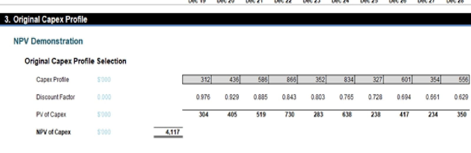
With cashflows and discount factors now known, calculating the Net Present Value of the original profile is straightforward, viz.

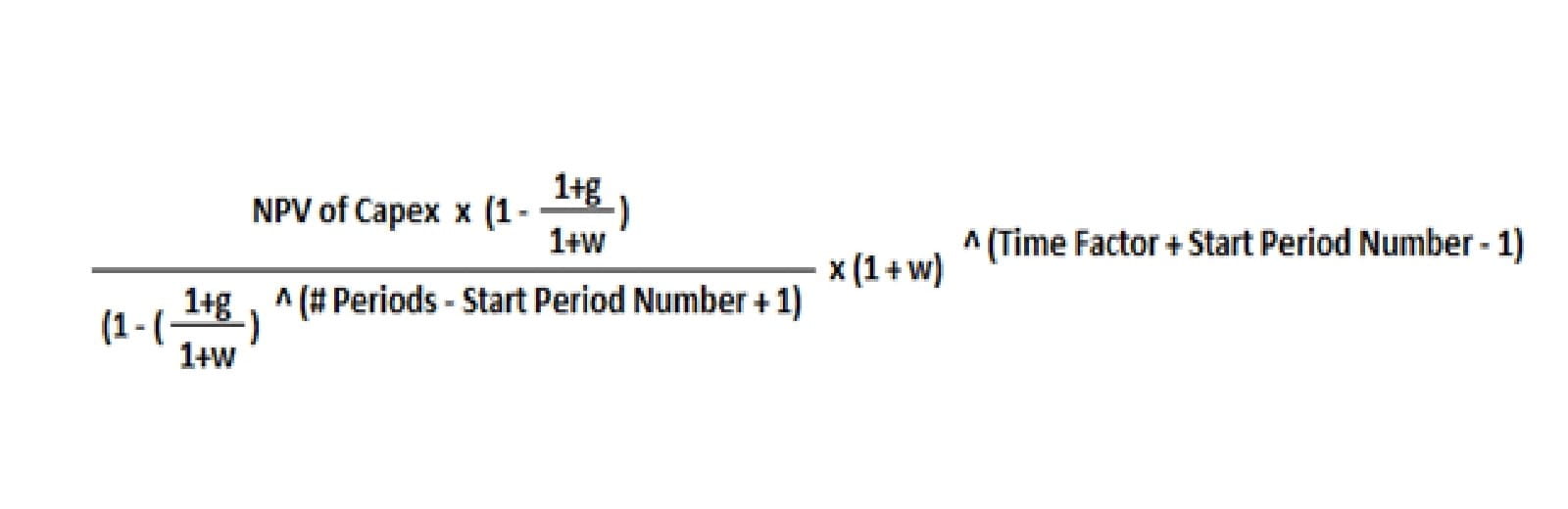
Now comes the tough part.  I need to replace this capex profile, with a “smoothed” equivalent, where I calculate an amount for the first period, grow it by the Growth_Rate for the same number of periods and yet still get the same NPV.  To do that I need to use the following generic formula to get the base capex figure to use:

Any questions!?  You have?  Oh sorry, we seem to have run out of time…

Most of the variables in this formula are self-explanatory, but just to be clear, g is the Growth_Rate and w is the Discount_Rate (cited as w as often this is the Weighted Average Cost of Capital or WACC for short). The exponent (1+g)/(1+w) appears a couple of times, so I have taken this into account when computing this in our Excel example:

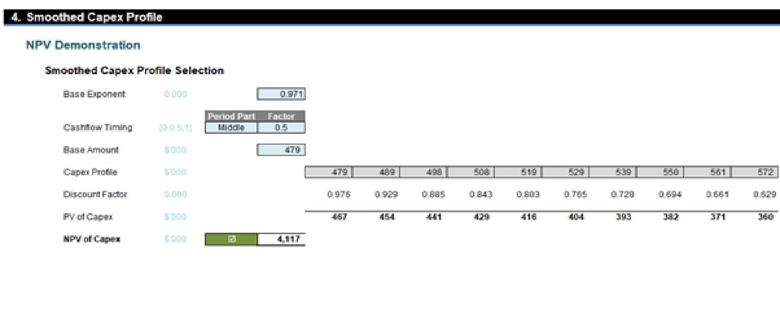
The Base Exponent (pictured above) is simply

=(1+Growth_Rate)/(1+Discount_Rate)

and the Timing_Factor is 0, 0.5 or 1, depending upon whether cashflows occur at the start, the middle or the end of each period.  The key formula is the Base Amount, which is a simplification of the horror formula above:

=(NPV_of_Original_Capex_Profile*(1-Base_Exponent)/

(1-(Base_Exponent^Number_of_Periods)))*(1+Discount_Rate)^Timing_Factor

This is then multiplied by the (1+Growth_Rate) for each period after the first in the NPV calculation, and the discount rates and NPV calculation are then simply as before.  This will give the same NPV – and I have even included a check to verify this.

There you have it: a profile you may use instead of your “erratic actual” one, which can compute the capex number to include in the terminal value (in this instance, it would be the final period value of 572, rather than the original 556).

Word to the Wise

This article is not intended to be a comprehensive discussion on valuations.  It is useful to calculate smoothed capex, not just for valuations, but also when normalising financial data for analysis purposes, for example.

This technique will only work when all periods are equal in length and percentage rates are converted to the rates for the period in question (e.g. monthly, quarterly, annually).  The Growth_Rate used should ideally be the one used in the terminal value calculations (where applicable); the argument for the Discount_Rate, however, is less well-defined.

If these conditions are not meant, using NPV to generate an equivalent Base Amount is still a reasonable technique.  Instead of using the formula above, you may need to use Goal Seek as an alternative.