
The Microsoft Research Blog discussed LAMBDA at the beginning of the year. They highlighted the power of this new Office 365 (Beta) function with this particular example:
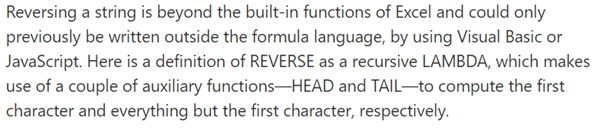
Aside from the fact that there is a mistake in the formula for REVERSE, having one too many closed brackets, the Research Team has erroneously stated that “…reversing a string is beyond the built-in functions of Excel and could only previously (sic) be written outside the formula language…”.
This is not true. Even if you haven’t access to LAMBDA and several other Excel 365-specific goodies, don’t worry – you can keep reading!
Consider the following:

For all current versions of Excel (not just Office 365, Excel on the web and Insider / Beta variants), I wish to write a formula that will reverse the text in a cell (i.e. reverse the text string). Since I want it to work “everywhere”, I cannot use VBA, dynamic arrays, JavaScript, TypeScript or Office Scripts.
It’s always dangerous to state that you can’t do something in Excel. No disrespect is intended upon the authors of the Microsoft Research article, but I have often found you may do just about anything in Excel with a little experience and, ahem, “imagination”. After all, necessity is often the mother of invention!
Having stated you might need an extended knowledge of functions and some innovation, it’s amazing what may be achieved with a little brute force and ignorance. We are still going to need several functions though...
The first one, LEN(text), gives the length of text in terms of the number of characters contained within the text string (including blank spaces), e.g.
=LEN("Mary Had a Little LAMBDA")
has a value of 24, being the total number of characters in the text string, including the total number of spaces between words. I imagine at this point you are probably not sure where I am going with this, but before I explain, perhaps I need to introduce the next function, INDIRECT, in a little more detail.
Excel’s INDIRECT function allows the creation of a formula by referring to the contents of the argument (cell), rather than the cell reference itself.
INDIRECT(ref_text, [a1])
The function syntax has two arguments:
- ref_text: this is a required reference to a cell that contains an A1-style reference, an R1C1-style reference, a name defined as a reference or a reference to a cell as a text string. If ref_text is not a valid cell reference, INDIRECT returns the #REF! error value. If ref_text refers to another workbook (an external reference), the other workbook must be open. If the source workbook is not open, INDIRECT again returns the #REF! error value
- [a1]: this is optional (hence the square brackets) and represents a logical value that specifies what type of reference is contained in the cell ref_text. If a1 is TRUE or omitted, ref_text is interpreted as an A1-style reference. If a1 is FALSE, ref_text is interpreted as an R1C1-style reference.
Essentially, INDIRECT works as follows:
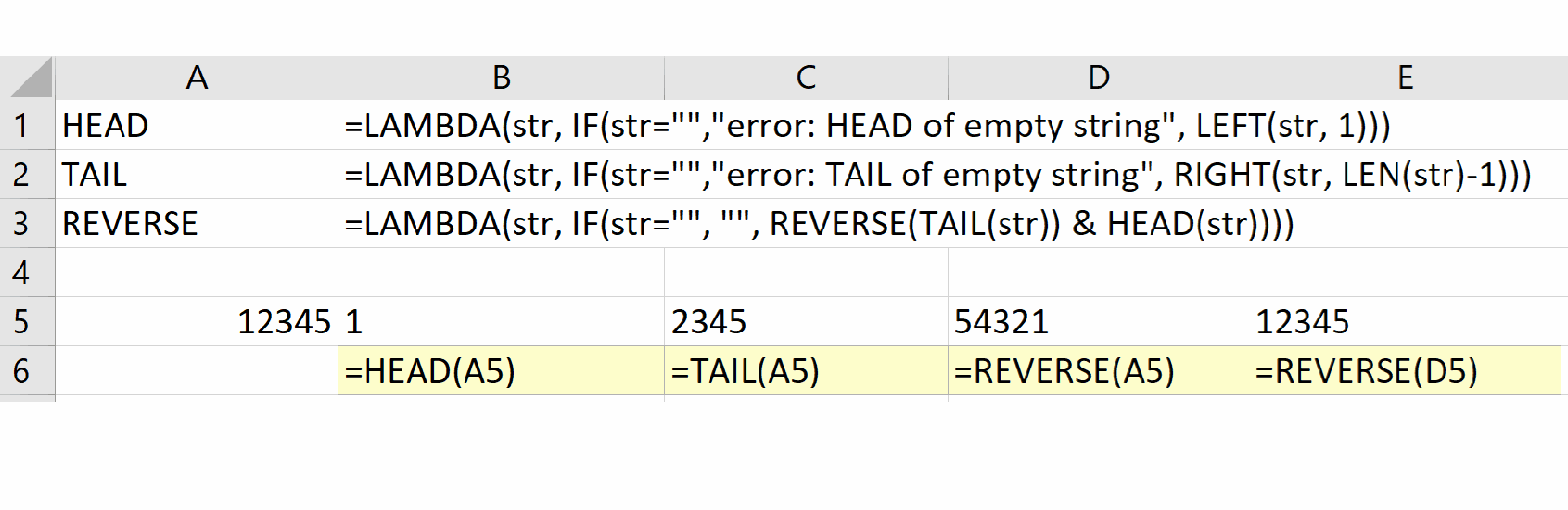
In the above example, the formula in cell D6 (the blue cell) is
=INDIRECT(D2).
With only one argument in this function, INDIRECT assumes the A1 cell notation (e.g. the cell in the third row fourth column is cell D3). Note that the value in cell D2 is D4, so this formula returns the value / contents of cell D4, i.e. 77.
This idea can be extended: the value indirectly referred to does not need to be in the same worksheet (or even workbook), or may even be of another type altogether.
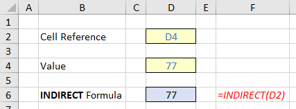
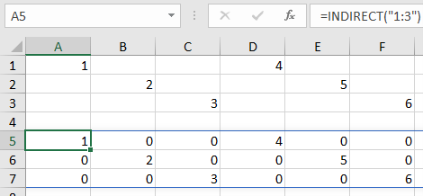
Let’s consider =INDIRECT(1). This would return #REF! because the intermediary reference 1 is meaningless in Excel. Yes, it constitutes a value, but INDIRECT is looking for a cell / range reference. You might think =INDIRECT(1:3) would reference rows 1 to 3 in Excel, but you would be wrong:
This is incorrect syntax. It needs to be =INDIRECT(“1:3”) because INDIRECT is expecting to convert text to a reference it can resolve, viz.
Hang on a minute: this is spilling – we are using dynamic arrays, and this won’t work in all versions of Excel. Well, yes and no; you may use =INDIRECT(“1:3”) in all current versions of Excel, it’s just this formula cannot be rendered in all versions. But that’s not what we want in any case.
Now, let’s extend the idea. Let’s consider =ROW(INDIRECT(“1:3”)):
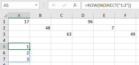
I have deliberately changed the occasional values in rows 1 to 3 to demonstrate that this has nothing to do whatsoever with the contents of rows 1 to 3. It’s generating the numbers 1, 2 and 3 as ROW(1) equals 1, ROW(2) equals 2 and ROW(3) equals 3. The ROW function has essentially passed the range argument “1:3” to whatever function or operation it has been set up for.
Just for completion and in case you are wondering, I cannot use COLUMN:
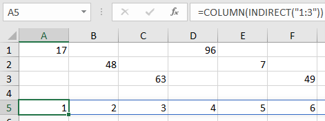
This would always extend to 16,384 columns (!).
If I combine this result with LEN from earlier,
=ROW(INDIRECT("1:"&LEN("Mary Had a Little LAMBDA")))
I would get
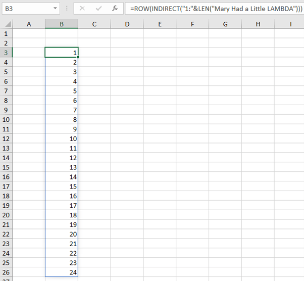
(The & operator simply joins arguments together.)
As I say, the list of the numbers 1 to 24 might not display in all versions of Excel, but the calculation engine would recognise the list. I can even reverse the order:
The formula
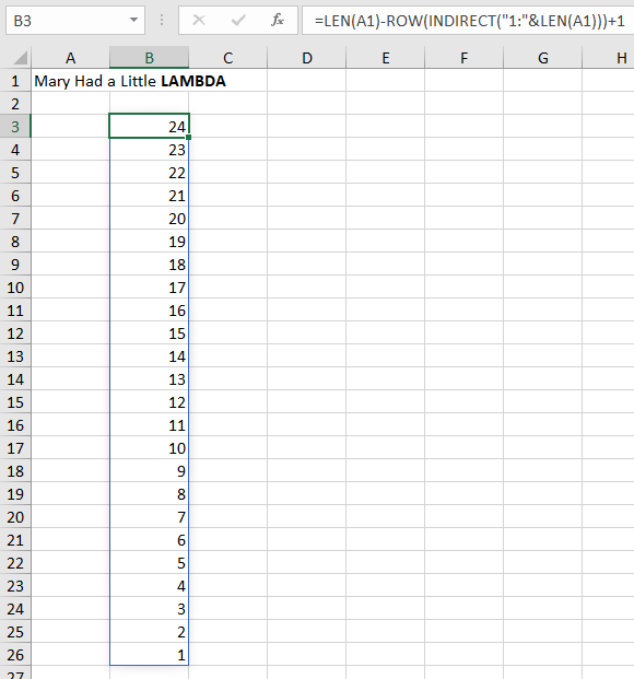
=LEN(A1)-ROW(INDIRECT("1:"&LEN(A1)))+1
takes the list generated earlier (ROW(INDIRECT("1:"&LEN(A1)))) and subtracts it from the length of the text string in cell A1 and adds one [1]. The first number would be 24 – 1 + 1 = 24, the second would be 24 – 2 + 1 = 23, the third would be 24 – 3 + 1 = 22, and so on.
Now I am ready to introduce my next function.
The MID function returns a specific number of characters from a text string, starting at the position you cite, based upon the number of characters you specify.
The MID function employs the following syntax to operate:
MID(text, start_number, number_of_characters)
The MID function has the following arguments:
- text: this is required and represents the text string that contains the characters you want to extract
- start_number: this is also required and specifies the position of the first character you want to extract from text. The first character in text has start_number 1, and so on
- number_of_characters: this argument is mandatory too and specifies the number of characters you want MID to return from the text.
It should be further noted that:
- if start_number is greater than the length of text, MID returns "" (empty text)
- if start_number is less than the length of text, but start_number plus number_of_characters exceeds the length of text, MID returns the characters up to the end of text
- if start_number is less than 1, MID returns the #VALUE! error value
- if number_of_characters is negative, MID returns the #VALUE! error value.
As an example,
=MID(“Mary Had a Little LAMBDA”,12,6)
would return the text string “Little”, being the sub-text string starting at the 12th character, consisting of six [6] characters.
It starts to come together now. Consider
=MID(A1,LEN(A1)-ROW(INDIRECT("1:"&LEN(A1)))+1,1)
in our above example:
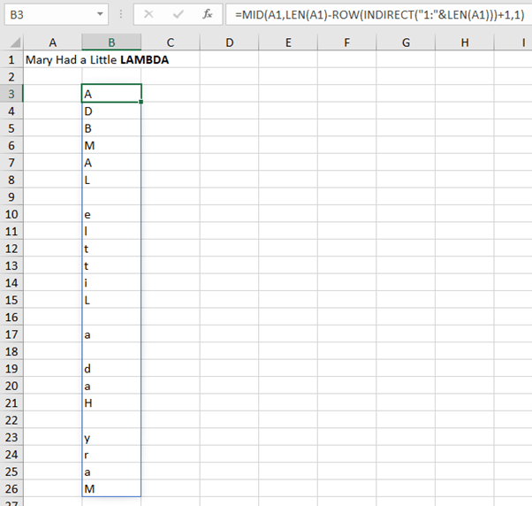
Each cell takes the nth character in the reverse list from the text string in cell A1. We simply need to join it together.
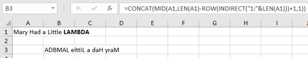
=CONCAT(MID(A1,LEN(A1)-ROW(INDIRECT("1:"&LEN(A1)))+1,1))
The CONCAT function replaces the old CONCATENATE function and combines the text from multiple ranges and / or text strings:
CONCAT(text1, [text2],…)
where text1 is the text item to be joined and text2 (onwards) are the additional items to be joined.
This is why you don’t need to worry about spilling: we do not require our result to spill, and we are not using any dynamic array functions.
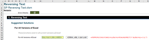
The associated Excel file provides this example, and also shows alternative solutions using dynamic arrays and even a LAMBDA function (or three).
Word to the Wise
In some versions of Excel, you may need to enter this formula using CTRL + SHIFT + ENTER, but even with older versions, this requirement should be unnecessary.
Archive and Knowledge Base
This archive of Excel Community content from the ION platform will allow you to read the content of the articles but the functionality on the pages is limited. The ION search box, tags and navigation buttons on the archived pages will not work. Pages will load more slowly than a live website. You may be able to follow links to other articles but if this does not work, please return to the archive search. You can also search our Knowledge Base for access to all articles, new and archived, organised by topic.
About the author

Liam has over 30 years’ experience in financial model development / auditing, valuations, M&A, strategy, training and consultancy. He has considerable experience in many different sectors (e.g. banking, energy, media, mining, oil and gas, private equity, transport and utilities). He is a regular contributor to the ICAEW, ICAA, CPAA, CIMA, Finance 3.0 and various LinkedIn specialist discussion groups. He is also an experienced facilitator for ICAA. Liam is a Fellow of the ICAEW, a Fellow of CIMA and is a professional mathematician.