Highest invoices by customer using Power Query

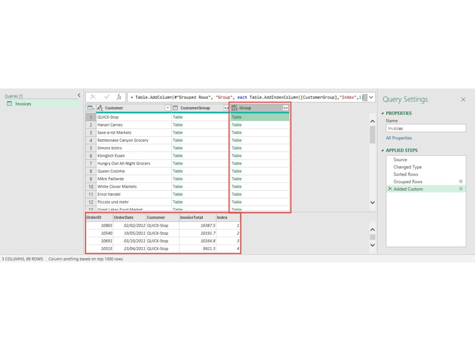
My chosen approach used the ability of Power Query to add an index column, combined with the Group By option. In this example, we have some basic invoice information including the customers' name and the value for each line of the invoices:

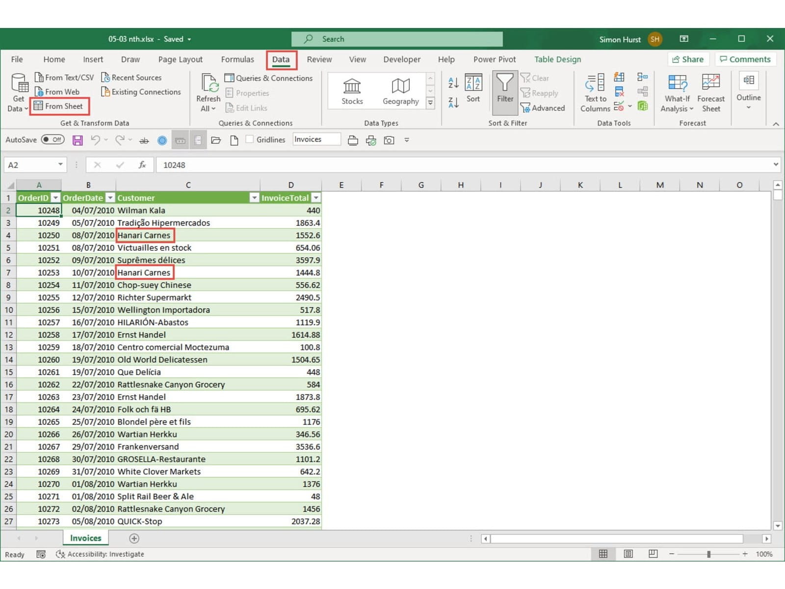
Liam's article showed how to return the position in the list of, for example, the second invoice for the client Hanari Carnes. We will take this a bit further with Power Query to show a table of the top three highest value invoices for each of our clients. As usual with Power Query, there are many different ways to address this problem so, if you have come up with a better one, please let us know at excel@icaew.com.

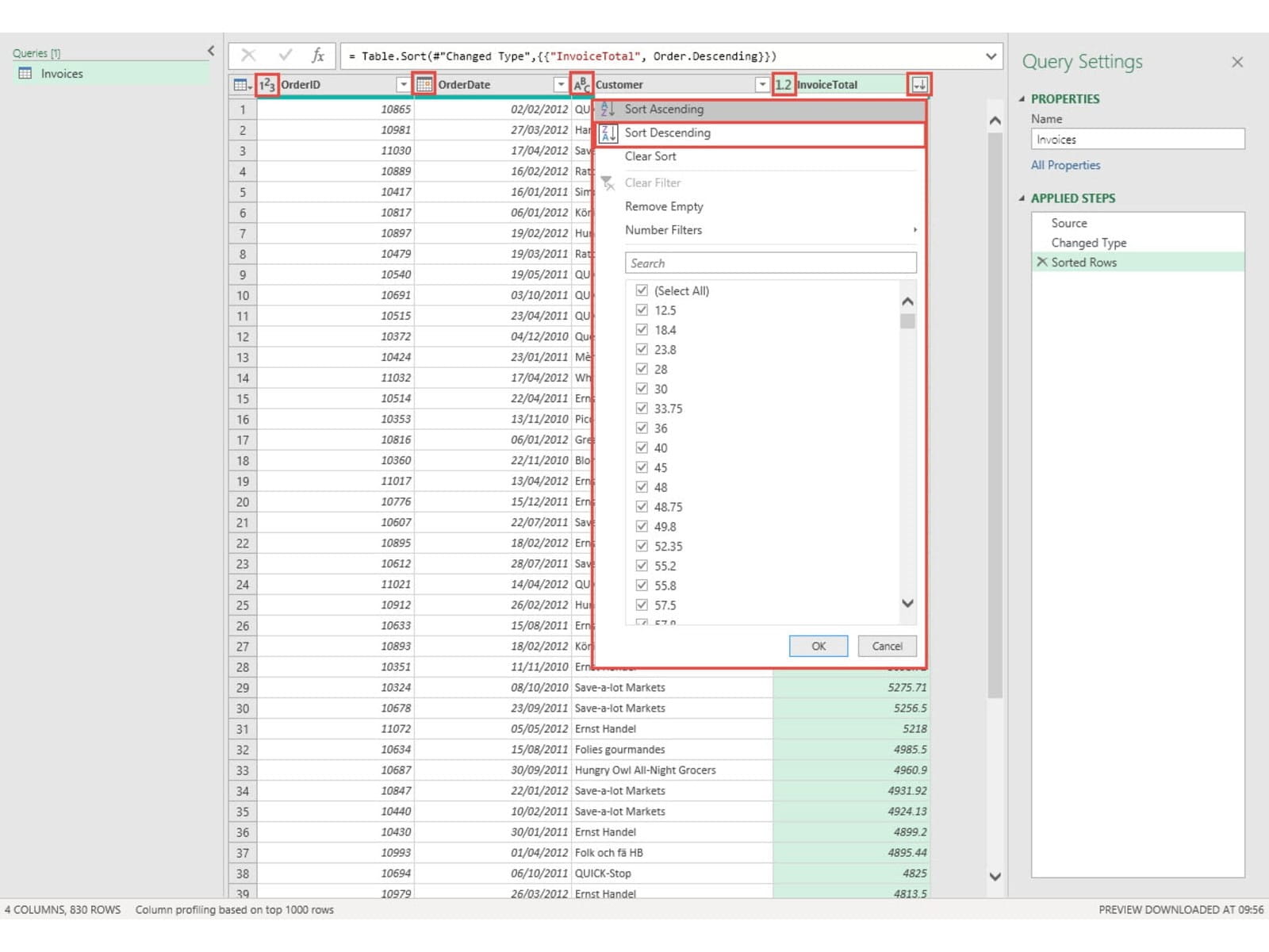
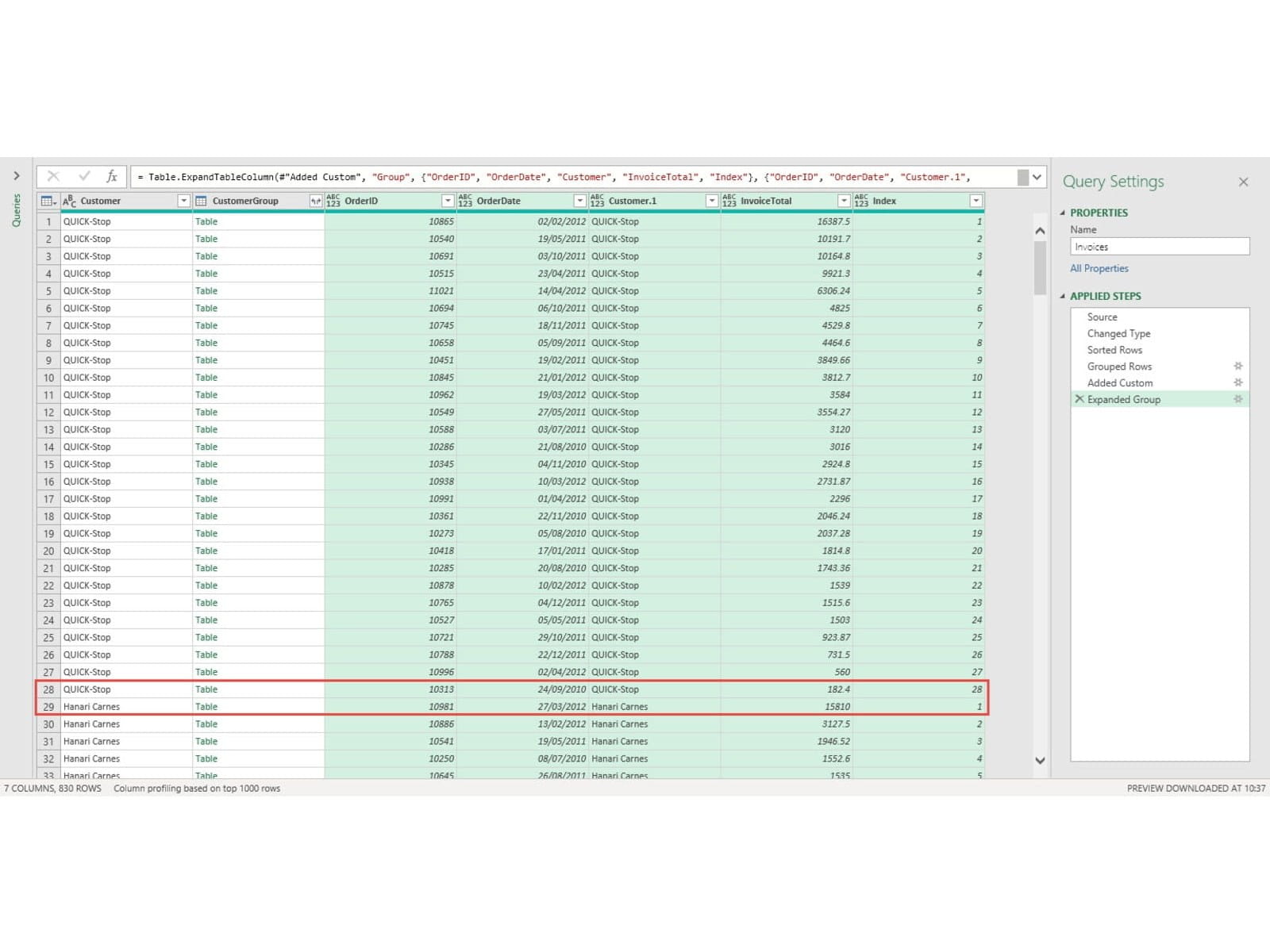
We'll start by using the Data Ribbon tab, Get & Transform Date group, From Sheet command to load our data into the Power Query editor. As revealed in a previous post this command has recently been renamed, having formerly been From Table/Range and, before that, From Table. Having loaded our data into the editor we will first check the data type for each column and, where necessary, change to the most appropriate type using the Data Type icon in each column header. Next, because we want to rank our invoices by value, we will sort by our InvoiceTotal column in Descending order:

We then need to rank our invoices within each customer. For simplicity, we will assume that we will ignore ties and just include any top three invoices, possibly excluding other invoices of equal value. To do this, we will first group our rows by Customer using the Transform Ribbon tab, Table group, 'Group by' command. We will group by our Customer column, give our new column the name CustomerGroup and, rather than choosing one of the aggregation Operations, we will choose the All Rows operation. This will create a new column, each row of which will contain a Table with all the rows for each of our customers. Here, we have clicked in the white space at the right of the new column in the first row to show a preview of the contents of the Table in that row:

Next, we add an index that runs across each group. We will do this by using the Add Column Ribbon tab, General group, Custom Column command. We need to create our index column by using a Power Query function but, as Power Query now includes AutoComplete for functions, this is very similar to creating a function in an Excel cell. One main difference is that Power Query is case sensitive, so the capitalisation within function names and also object names (such as a column name) must be respected. Here we have called our new column 'Group' and used the Table.AddIndexColumn function to create, from our CustomerGroup column, a column that we have named as Index and that starts from the number 1, with a default increment of 1:

Note that, at the bottom of the Custom Column dialog, a check appears to show us whether our function has been correctly entered, or the nature of any error. Having added our closing right Parenthesis and clicked on OK, another column of Tables is created, this time with our new Index column added:

We can use the Expand button at the left of the header of this column to expand our column to include all the rows and columns that we need. As we can see, the Index restarts for each customer:

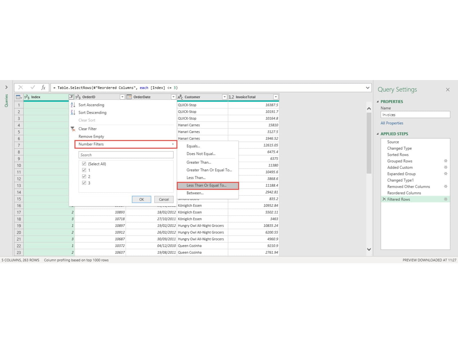
Now we can just revisit our Data Types, remove redundant columns and change the column order before setting a filter on our Index column to only show items Less Than Or Equal To 3:

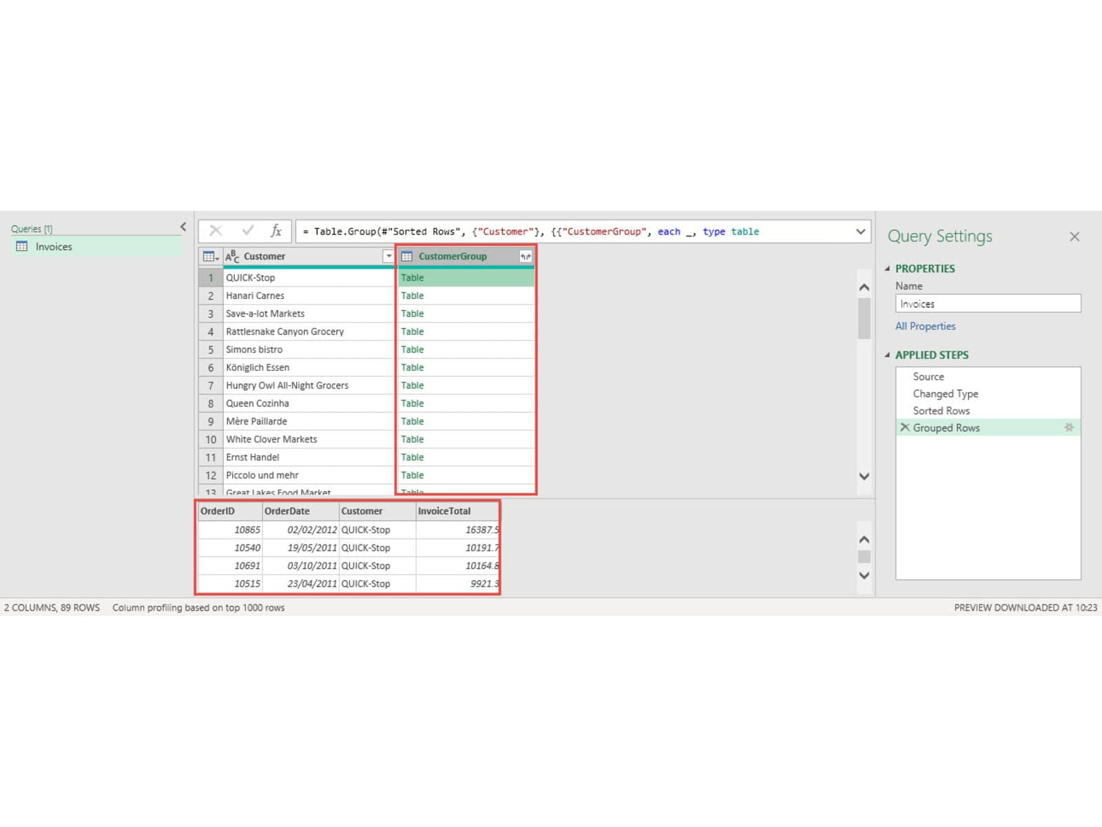
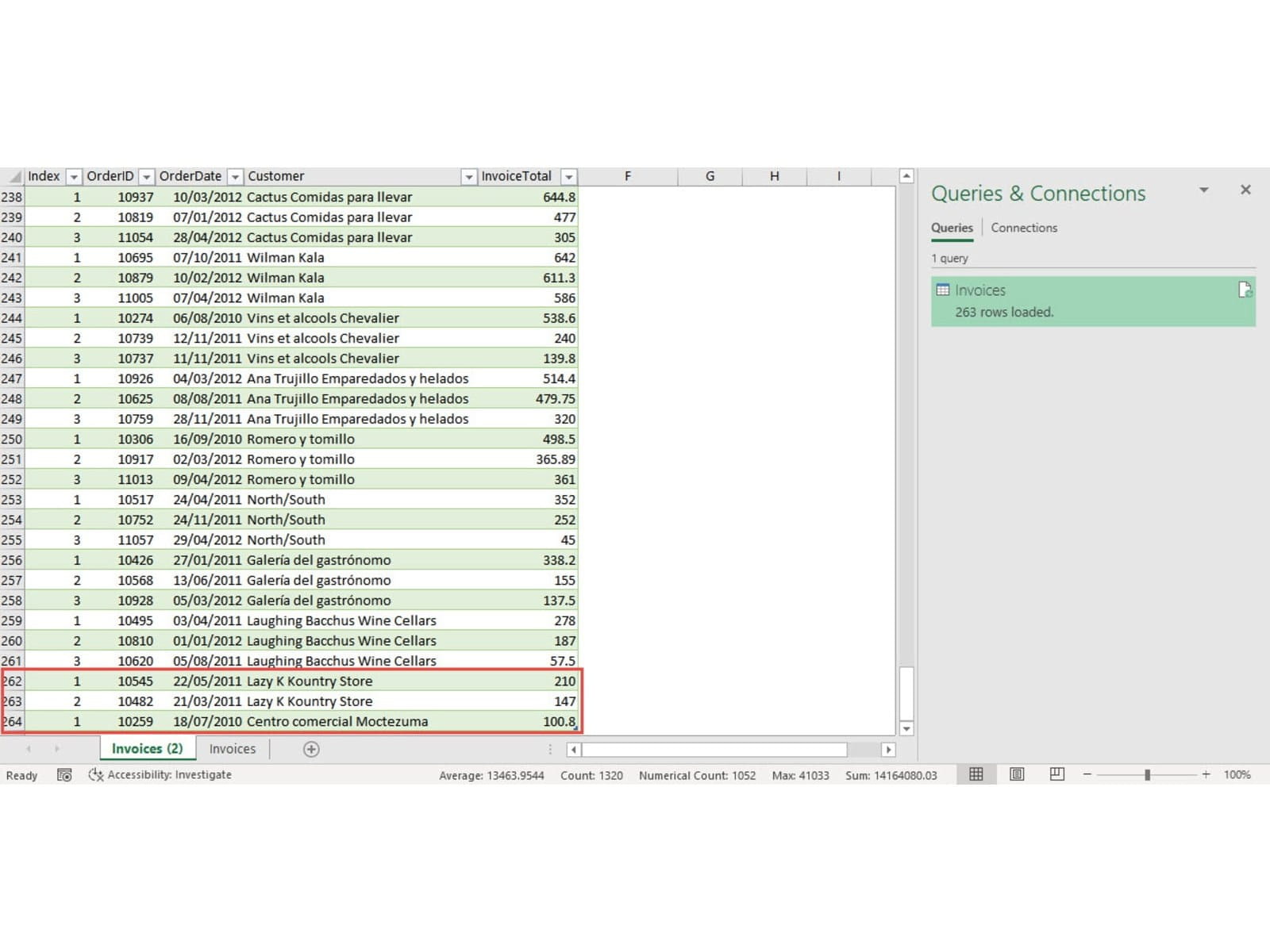
This gives us our list of the top three highest value invoices by Customer and we can use Home Ribbon tab, Close group, Close & Load to load this table into an Excel worksheet. At the bottom of our table, we can see that our last two customers only had 2 and 1 invoices respectively:

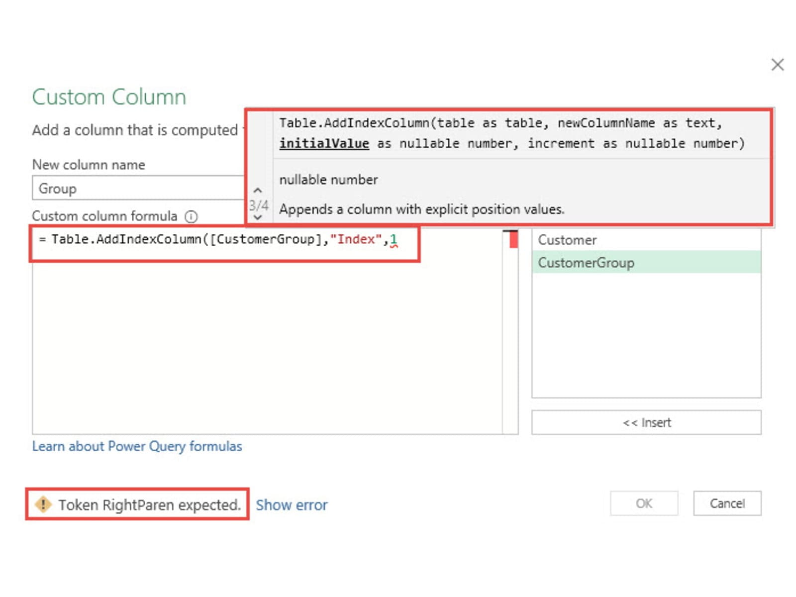
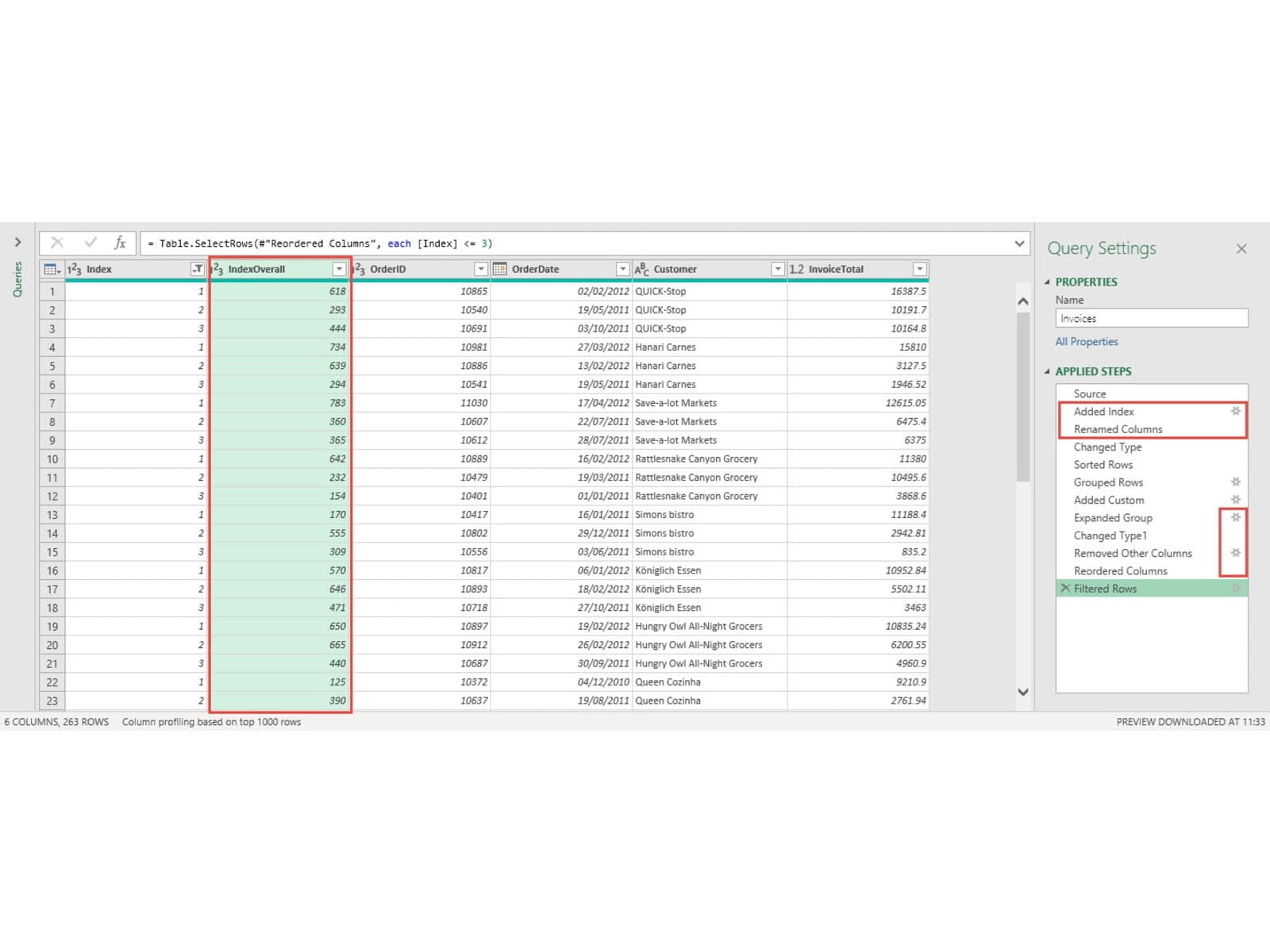
Of course, we still haven't achieved what the formula approach did, the display of the position of the Nth item in the group. We could just go back and edit our query to add an overall index column right after our Source step and then edit our 'Expand' and 'Remove Other Columns' and 'Reordered Columns' steps to add this to our output table: