
I was writing my latest contribution to Chartech recently when I discovered something about Linked Pictures that I hadn’t previously realised. I was using the Excel Linked Picture object to automatically pick the member of the sales team that had the highest value of sales, and display their picture.
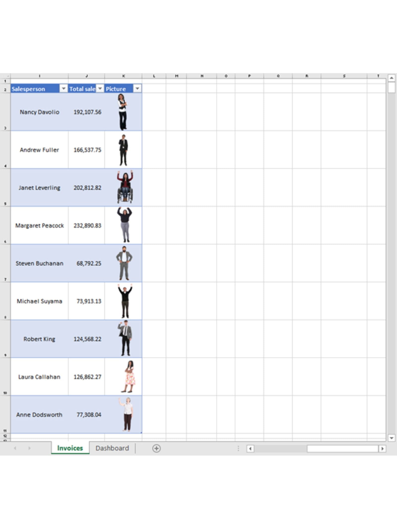
The basic approach was to create an Excel Table that included the sales team members’ names, sales values achieved and their picture. The cell row and column dimensions were changed so that, for the picture column, each picture could be sized to fit in a single cell:
There are two main ways to create a Linked Picture. You can add the Excel Camera tool to the Quick Access Toolbar, or the Ribbon, and then select the cell or cells that you want to take a picture of, before clicking the Camera and then clicking elsewhere to create a separate Picture object that has the selected cell or cells as its source. Alternatively, you can just copy the source cell or cells and then use Paste Special, Linked Picture to achieve the same result without needing to use the Camera.
Although, as will become significant later, if the selected cell or cells include one or more cells that are within an Excel Table, you will need to use the Camera approach. In our case we will create a Linked Picture based on any one of our sales team picture cells. Once the Linked Picture has been created, when we select it, the source cell reference will show up in the Excel Formula Bar.
We can easily change the reference in the Formula Bar to refer to a different cell or block of cells. However, what we need to do is to create a dynamic reference so that our picture will automatically change to show the picture of the team member that has the maximum sales value.
We can do this in a variety of ways, but I chose to use the Excel
INDEX(), XMATCH() and MAX() functions: =INDEX(SalesTeam[Picture],XMATCH(MAX(SalesTeam[Total sales]),SalesTeam[Total sales])) Note that the default match mode for XMATCH() is exact, unlike its predecessor MATCH() which defaults to an approximate match.
Although, we can change the reference in the Formula bar to a different cell or cells, we can’t change to a formula that incorporates an Excel function without the reference being rejected as invalid. As is the case with several other objects in Excel that don’t allow the direct use of functions, we can overcome this by allocating our formula to an Excel Range Name and then use the reference to the Range Name as the source for our object. I have used this technique successfully in the past, but I couldn’t make it work properly this time. I kept getting ‘Reference isn’t valid’ error messages when I tried to enter the Range Name as the source reference.
Assuming that I had made an error in the formula I checked it thoroughly, tried to replace INDEX() MATCH() with OFFSET(), but still couldn’t make it work. The standard technique I use in this situation (after the swearing and keyboard thumping) is to rebuild the formula step-by-step, replacing functions with values and simplifying all the cell references. What happened next was the really confusing bit. I made it work with the very simplified approach then gradually restored all the functions and Table references and it still worked. Then I tried to apply the same Range Name to another Linked Picture and it was rejected with the ‘Reference isn’t valid’ error message. When I went back to the first picture and used Enter to accept the previously entered Range Name it was rejected, even though pressing Escape to leave the formula unchanged, referring to exactly the same Range Name, did still work.
I then leapt to a conclusion that turned out to be incorrect. I assumed that the Linked Object source was checking the formula ‘behind’ the Range Name when it was entered into the Formula Bar, finding that it contained one or more functions, and therefore rejecting it. However, if the Range Name had been allocated when the formula didn’t contain any functions it would be happily accepted and would remain working even if the formula were to be subsequently changed to include functions. This seemed to fit the current situation. Fortunately, I persevered with checking and ruled out the use of functions as the culprit. This left the use of Structured Table Language in the frame (appropriately enough). Unless anyone can prove otherwise (excel@icaew.com) it seems that you can’t allocate a formula as a Linked Picture source if it contains a Table reference.
However, if you create the Range Name formula using standard cell references it can be allocated as your Linked Picture source and you can then go back and change the formula back to using Table references and thus being more automatic. The Linked Picture source will continue to work. This means that if you do want to automate a Linked Picture with a formula that incorporates a Table reference you have to do it in this convoluted way, even if you just want the picture to be of an entire table, with no Excel functions involved. Although this hypothesis fits the facts as far as I’ve discovered them so far, it might not be the whole answer or even the correct answer. Please let us know using the above email address if you have come across a better solution.
Archive and Knowledge Base
This archive of Excel Community content from the ION platform will allow you to read the content of the articles but the functionality on the pages is limited. The ION search box, tags and navigation buttons on the archived pages will not work. Pages will load more slowly than a live website. You may be able to follow links to other articles but if this does not work, please return to the archive search. You can also search our Knowledge Base for access to all articles, new and archived, organised by topic.
