Debunking sampling myths

Finance professionals are not usually required to be statisticians, but we do acquire and analyse data, and sometimes need to think about how far we can generalise from that data. At times we might decide against a simple survey or other data-gathering exercise because we overestimate the amount of data needed for a reliable conclusion. At other times we may err the other way and generalise too far.

People often overestimate the sample size needed for surveys. Typically, they think a sample of several hundred is needed when in fact fewer than 100 would be enough. One reason for this is the tendency to think that samples need to be a particular percentage of the population sampled. You might even see samples expressed as a percentage of the population.

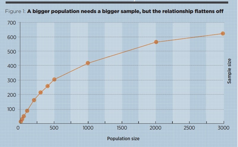
It is true that larger populations need larger samples for the same level of confidence, but in percentage terms the sample gets rapidly smaller as the population increases, and eventually there is no appreciable gain from a larger sample.

To illustrate, imagine you want to establish an error rate so that you are at least 95% confident the true error rate lies within plus or minus 5% of your best estimate. This is quite a high level of confidence and requires a fairly large sample (for this illustration I have gone back to first principles and simulated sampling using Bayes Theorem rather than using a sample sizing formula).

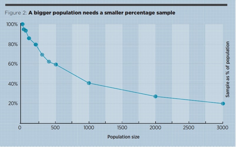
Figure 1 shows how the sample size, needed to maintain confidence, grows with population size. Figure 2 shows that the sample as a percentage of the population starts at 100% but soon dwindles to less than 20%. Later in this article we will see a sample that does not get beyond 14, ever.

It is a myth that the sample size needs to be a fixed proportion of the population. 

Another cause of overestimating the required sample is typified by three myths.

1. Statistical confidence is solely driven by the sample size.
2. Sample sizes can and should be calculated before doing a study.
3. The confidence level sought should always be 95%.

In fact, the confidence you get from a sample also depends on the type of conclusion you want to draw and on the reality of the data. It is true that you should make some sensible estimates to help you plan your research, but those estimates will inevitably involve guessing what the results of your research will be.

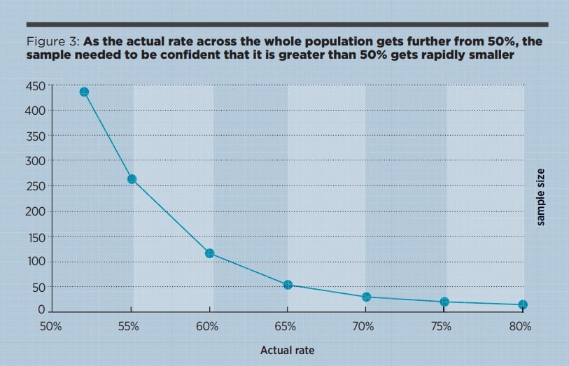
The general principle is that the finer the distinction you want to make, the bigger the sample needs to be. To illustrate, suppose you plan a poll to find out which of two products is preferred. You can only choose one product to invest in so you will choose the preferred product and ignore the other, regardless of the strength of preference. Figure 3 shows how the sample size (to be 95% sure product A is preferred) varies with the actual rate of preference in the population. I’ve assumed a population of 500 and used a simulation again.

When the true preference across the whole population is 80% you only need to test 14 items on average to be 95% sure of the majority. When the true preference is just 52% then you need to test nearly the entire population. Incidentally, that 14-item sample is still about equally convincing if the population is 3,000 instead of 500 – population size increases make almost no difference.

Back when I was an external auditor an unusual regulatory audit was requested and the client wanted to know what sample size should be tested to be 95% sure the error rate of a process was no more than 3%. This sounds impressively statistical but showed a fundamental misunderstanding. The sample size needed would depend on the actual error rate of the process. If it was close to 3% we might need a huge sample. If it was actually greater than 3% then no sample would be big enough.

Many of the data points we deal with are really summaries of detail below, such as monthly totals. What difference does that make? It is a mistake to think that data points are just data points or to imagine that summaries contain all the information in the detail below.

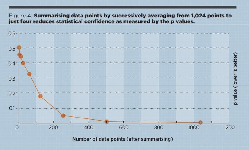
To illustrate, here’s what happens at different levels of aggregation when you do an ordinary regression of one variable onto another. An example of this would be trying to capture the relationship between sales effort and sales achieved across many sales people or teams. In this completely fictitious illustration (Figure 4) the most detailed level is with 1,024 data points; the next level has 512 points by just averaging two data points from the full detail; the next level has 256 points by summarising again, and so on.

In this illustration the models built using the full detail are much more reliable, and their statistical robustness (shown in Figure 4 by the lower p values) is far better when detail is retained. So if you think some variables are related, make a scatter plot and do regression using the least summarised values possible, not monthly or geographic totals or averages.

The power of modern statistical software can be intoxicating, and this leads to another rather common myth: the idea that regression with multiple predictor variables doesn’t require much more data than other procedures. The problem lies in the contrast between ideal and real-life datasets.

With ideal data the performance of even multiple linear regression (the simplest, most traditional option) is excellent, easily finding the weight of 10 drivers from just 20 cases. With 50 cases it comfortably deals with some non-linearity or some multi-collinearity – two imperfections that challenge linear regression.

And yet, despite this apparently amazing performance, I have found multiple regression to be a bag of nerves with most real datasets. The weights recovered are unreliable and influenced by data that should not have any effect; often, nothing useful is found.

To understand this we need to consider two factors that have a powerful effect on regression success: the number of variables that truly drive the output, and the number of those variables we use in the regression (as Figure 5 shows).

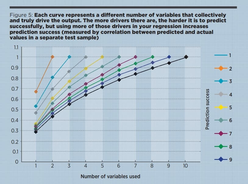
In most real-life regressions the outputs are, in truth, driven by many drivers and we have data for hardly any of them. That's why multiple regression is often disappointing.

In the illustration used to create Figure 5, I assumed that each driver was equally important to the output, but you can see that as the number of drivers grows, the importance of each individual driver shrinks.

If the drivers are not equally important and we are interested in one of the less important drivers, then the required sample size can shoot up. For example, if you try to find the weight of a factor and it is in fact just one tenth of the importance of each of the others, then the number of cases needed to estimate its importance jumps from 50 to nearer 5,000 (these are very rough figures just for illustration).

Another more subtle myth is the idea that the number of cases you need rises with the number of variables you use, so if you are struggling you can always cut some variables out of your model. In reality regression does better if it has data for more of the true drivers, even if this means dealing with more variables. The problem is not the number of variables you use but the number of variables that truly determine the output. It is better to use all you have that seem to be relevant.

Regression struggles when it lacks a full set of driver variables. If we then ask it to work out the importance of a minor variable then the cases needed for statistical confidence skyrocket. We need big data to stand a chance of learning something reliable.

Having said that many cases are needed to confidently estimate the weight of individual factors, things are very different for prediction accuracy. Here, using bigger data is not important and 50,000 cases are little better than 500. What really makes a difference is finding and using more of the variables that truly drive your target.

We have seen that sometimes the sample needed for useful conclusions is smaller than we might think, and sometimes larger. The number we really need can only be guessed in advance because it depends on what the truth is, and we only know that after analysing the data.

In general we will be more successful with statistical analysis if we study effects that are strong and clear, preserve detail, use values for more of the variables that are important, and are content with modest conclusions rather than trying to discover tiny points from variables that give only part of the picture.

Download pdf article:

• Debunking sampling myths
  Business & Management Magazine, Issue 252, March 2017

Full article is available to ICAEW members and students.

Further reading into sampling is available through the eBooks below.

Our eBooks are provided for ICAEW members, ACA students and other entitled users. Users are permitted to access, download, copy, or print out content from eBooks for their own research or study only, subject to the terms of use set by our suppliers and any restrictions imposed by individual publishers. Please see individual supplier pages for full terms of use.