
'How to' series
In this series we will be looking at the Excel tools and techniques that help you accomplish a range of day-to-day Excel tasks more efficiently and effectively.
As part of each article, we will be scouring the extensive Excel Community archive to provide links to additional details and ideas.
This is the story of the series so far:
- Excel how to: speed up entering formulae part 1 - using the dollar signs to fix all or part of a reference
- Excel how to: speed up entering formulae part 2 - using Range Names to make formulae easier to enter and understand
- Excel how to: speed up formulae - using Excel tables part 1 – creating dynamic references by referring to Table columns and using Table structured references to make formulae easier to understand
In our first look at Excel Tables, we concentrated on referring to Table contents from a cell outside of the Table itself. This time we will consider formulae within Tables.
Formulae in Table columns
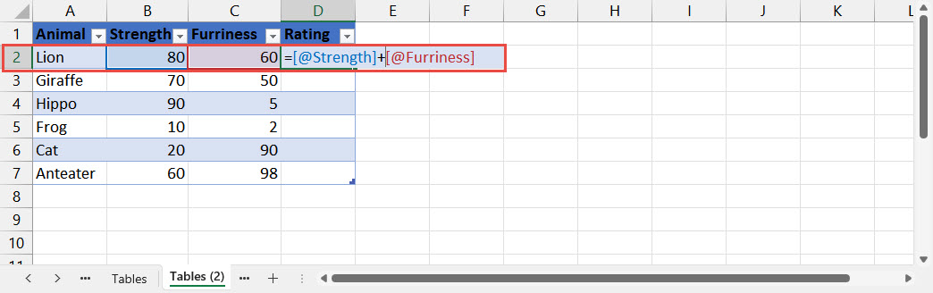
We will build on our example from the previous episode by adding a column to the right of our existing Table to hold a value for animal furriness. Just typing the column heading in cell C1 will cause our Table to expand to include our new column. Having entered our values, we will add a new ‘Rating’ column heading in D1. This column will contain an overall animal rating, calculated by adding strength and furriness. If we enter our formula in D2 by typing = then clicking on B1, typing +, then clicking on C1, Excel will create our formula using Table structured references:
=[@Strength]+[@Furriness]
Note that, unlike when referring to a Table cell from outside of the Table, there is no need to specify the Table name in addition to the column name, and that the @ modifier has been used to refer to the current row for both columns:
One of the main ways to speed up formula entry is to not have to enter or copy each formula in the first place. AutoCorrect will automatically copy a formula entered into an empty Table column to all the other cells in that column. In addition, where we use a consistent, calculated column, our formula will automatically be copied down to any rows that we add to our Table.
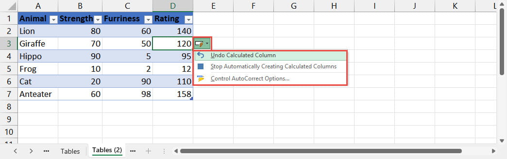
Although automatically copying our formula to the rest of the column is the default behaviour, it can be overridden using the AutoCorrect Option dropdown that pops up after the AutoCorrect operation is performed. The AutoCorrect, AutoFormat As You Type, options also allow you to turn the behaviour off altogether, with the Option dropdown including a short cut to doing this with the ‘Stop Automatically Creating Calculated Columns’ option. Although the default calculated column behaviour makes it quicker to set up a consistent formula in an entire Table column, it doesn’t force the formulae to stay consistent. Were you to change one of the formulae in a calculated column, the default would be to overwrite the existing formulae with the new one, but choosing Undo Calculated Column from the Option dropdown would leave the existing formula in all the other column cells:
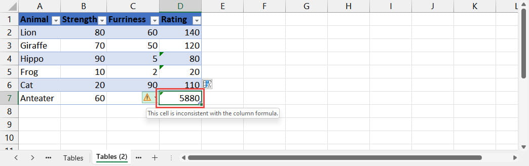
Subject to the Excel Error Checking options, inconsistent formulae in a Table column should be highlighted as shown above. Note that this error checking behaviour is significantly different within Tables compared to simple ranges:
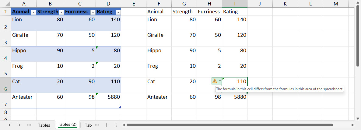
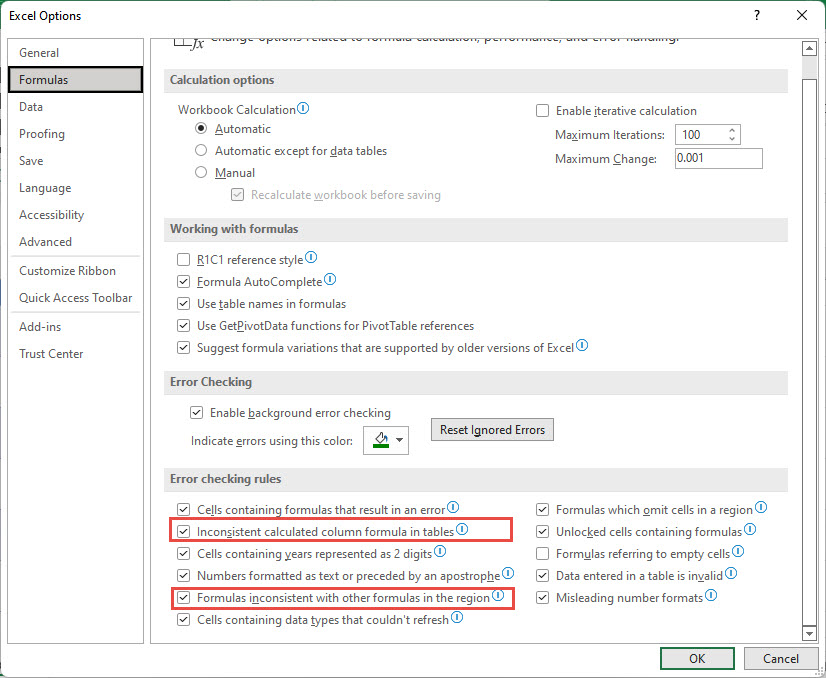
In the simple range, cell I4 is not highlighted as an error because it contains a value and not a formula, cell I7 is not highlighted because it is at the end of the range, and therefore is not surrounded by other formulae. Also. in the range, Excel decides that cell I8 is the formula that differs from adjacent formulae. The two different types of error checks in operation can be seen in the Excel Options, Formulas, Error checking rules section:
So, we can see that the use of Tables for calculating columns can do the work of copying formulae for us; helps avoid, but does not prevent, formulae in a column being inconsistent and highlights more inconsistencies than when the calculated column is just part of a simple range.
One formula to demonstrate them all
We can bring many of the areas that we have covered in this, and the previous article, in the following example. This might seem complicated but does demonstrate many of the Structured Reference features that we have covered across the two articles.
Here, we want our totals to appear in separate columns for each month. We have entered the month end date as the column heading for three of our columns:
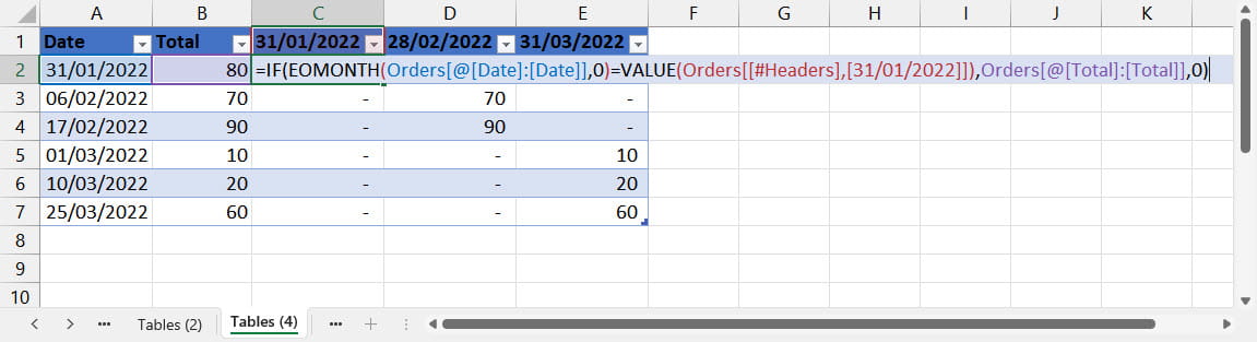
The formula entered into cell C2 is:
=IF(EOMONTH(Orders[@[Date]:[Date]],0)=VALUE(Orders[[#Headers],[31/01/2022]]),Orders[@[Total]:[Total]],0)
We are using an IF() function to check whether the date of each row falls within the relevant month. The EOMONTH() function converts the dates in our Date column to the month end of the same month. Column headers in Tables cannot be entered as formulae and are treated as text rather than numbers or dates so, for our IF() comparison to work, we have to use the VALUE() function to convert our header value to a valid date. Where our dates match, IF() returns the value in the Total column for that row, and returns zero if not.
The complication arises because we want to create a single formula and copy that formula from our first date column across to the other two. However, our formula contains a combination of absolute and relative references. The references to the Date and Total columns need to stay the same in all three columns, but the reference to the header value needs to change for each column. For this reason, we can’t just use the Control+r for ‘right fill’ shortcut we used in the previous article as this would not change our column header references. If we just created a ‘normal’ reference to the Date and Total columns, this would change when copied across. Accordingly, we have used the single item range reference to fix those references, so that we can just copy the formulae in column C across to columns D and E:
Orders[@[Date]:[Date]]
The easiest way to enter this rather odd part of the formula is probably to create a normal range of Orders[@[Date]:[Total]] as part of the formula by using the mouse to select the two cells involved, and then to overtype ’Total’ with ‘Date’. Note than when referring to a range, the reference includes the Table name as well as the column name(s).
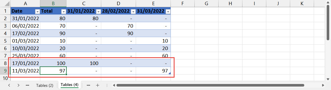
Below, we have added a couple more rows and can see that the formulae in our three calculated columns are automatically copied to our new rows:
Related links
Archive and Knowledge Base
This archive of Excel Community content from the ION platform will allow you to read the content of the articles but the functionality on the pages is limited. The ION search box, tags and navigation buttons on the archived pages will not work. Pages will load more slowly than a live website. You may be able to follow links to other articles but if this does not work, please return to the archive search. You can also search our Knowledge Base for access to all articles, new and archived, organised by topic.
