Live Q&A 3 – ALL your questions answered!

How can I sort and make subheadings for these groups for example, from a nominal ledger of donations received, group them by donor name and subtotal?

The simplest way is to make a PivotTable with Insert => PivotTable.

You can also create automatic groupings of data like this by sorting the data and using Data => Subtotal.

How can I better manage a lot of text data (not numbers) which varies slightly in each cell and has been manually added in? Colour cells, filters?

Text data is definitely harder to work with. Consider using an Excel Table (Home ribbon or Ctrl T) to manage data more easily. Reducing variability from manual entry is a good idea, too – consider using data validation to e.g. force users to input from a defined list of options.

Is it true that the IFS formula only works on Office 365?

It’s also in Excel 2019.

The function is designed to replace nested IF functions; it takes the first TRUE result from a list of tests and outputs the result:

=IFS(test 1, output 1, test 2, output 2, test 3, output 3…)

Can I sum with XLOOKUP? I have a dump of timesheet entries, several rows per person each with a time entry. I want to be able to sum per person, per class of time entry listed in one particular column, time values listed in an adjacent column.

You could, but a PivotTable would probably be the easiest option here.

Do you know of any websites which provide exercises for excel skills e.g. functions; pivot tables etc.? Even if they are at a cost.

You’re in the right place! Learn more about the Excel Community and its online training at www.icaew.com/joinexcel.

If I have a table that had pivot tables applied, how do I break them down to figure out how the person before me categorized them?

You can double click on any value in a PivotTable to see a report breaking down that total.

Templates: I wish to change my "normal" template but how do I find exactly where they are stored etc?

You can change the templates that Excel uses when creating new workbooks / worksheets by creating a new file and saving as an a .xltx (Excel Template) file – selecting this file type should automatically redirect your Excel to save in the appropriate folder for workbook templates. New sheets are created from a template called Sheet in the XLSTART folder.

On an excel transcript of bank statements including payments and receipts, is there a feature to subanalyse each receipt/expense category -e.g. rental income, bank charges - etc. into separate columns?

You could break the amounts into columns by using an IF, e.g.:

I have been asked if there's an efficient way of keeping records of pledges in a charity. So donors pledging money to the charity and obviously we don't want input in the accounts as the money hasn’t been received yet.

I would just add a column in your donation tracking sheet that notes whether amounts are donations received or pledges, and update as appropriate once pledges actually materialised.

I struggle with how to use look ups. I often have two spreadsheets with different information about the same entity, identified by a reference number. I want to be able to pull information from one spreadsheet into the other. I assume this is lookups but I can't seem to make it work for me.

Lookup functions are an essential Excel skill whenever you are pulling data from one location to another based on a unique identifier. There are three main functions used: VLOOKUP, INDEX MATCH, and XLOOKUP. VLOOKUP is the most commonly used but is a bit clunky, as it requires the identifiers to be on the left of the table:

=VLOOKUP(identifier to look for, entire table to search, column number desired, FALSE)

INDEX MATCH is more flexible and more reliable:

=INDEX(column desired, MATCH(identifier, column of identifiers, 0))

XLOOKUP is the easiest and best but only available in Office 365:

=XLOOKUP(identifier, column of identifiers, desired output column)

How do you update/change the data range which a pivot table looks at?

Select the PivotTable and use PivotTable Analyze => Select Data Source. Using an Excel Table as the source should prevent most cases where you need to do this.

How do you maintain formatting in a pivot table after refreshing?

Set the formats by selecting the value field => Value Field Options => Number format.

How to show on a bar chart an average line horizontally?

Create an additional column in your data with the average value and then set your chart type as a combo chart, with the values as a bar chart and the average as a line chart:

Issue with pivot tables.... when I roll forward a workbook and "save as" a new month say the pivot tables still look at the old save file rather than the same sheets in the new workbook, which is horrible creating links between workbooks, is there anyway for the pivot table to always look at data area in the current workbook?

This is likely caused by however you are doing the roll forward – Pivots within one workbook should automatically move over to the new one unless something like saving a sheet at a time is happening.

With conditional formatting, e.g. If X is above 0, colour red, or X below 0 colour green, this works well, but there’s an issue that blank cells end up coloured and I would prefer these blank. How do we do this?

Separately, can you show me how you would make a conditional format for changing cell colour depending on two separate cell conditions e.g. Cell X above 0 and Cell Y = “Y”

These are both doable using Conditional Formatting => New Rule, and using a formula as the rule:

=AND(A1>0, A1<>“”)

=AND(A1>0, A2=”Y”)

If data is contained within only 2 or 3 columns but a large number of rows is there way to create a print page set up so that next set of print data "snakes " i.e. is to the right of the original columns to reduce number of print pages?

Unfortunately not – Excel printing isn’t that great and I tend to recommend against it.

What's the quickest way to sum cells across worksheets if each worksheet is in the same format?

You can do a “3D reference” such as:

=SUM(Sheet1:Sheet3!A1)

However be very careful using these – if any of the sheets change, or the worksheets are moved around, they break very easily.

How do I format date in an excel which is captured using various formats i.e. DDMMYYYY and MMDDYYYY in the same column?

You need to find a way to separate out the days, months, and years into separate columns, and then use DATE to recombine them. Watch out for dates like 04/05/2021 which are ambiguous and which will have already been converted by your Excel based on our locale settings.

Which formula tips do you have for forecasting models and switches? moving away from vlookups etc.?

I would recommend using something like an INDEX for picking a value based on a scenario number. There’s more detail in this Excel Tip of the Week post.

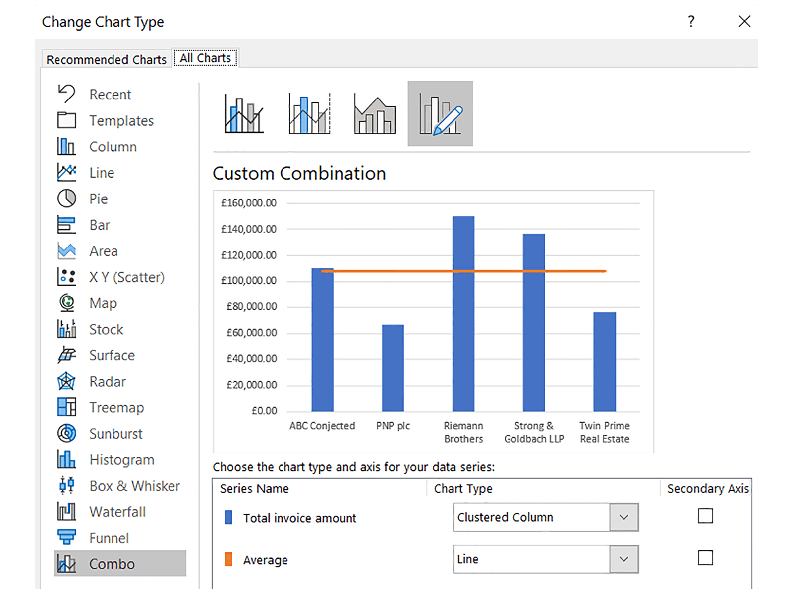
Is there an easy way to create tranche values based off a series of input values? i.e. if you wished to work out the amount of commission to be paid if commission % increased as value increase, so 5% on 0-500 6% on 500-1,000…?

Not easy, but a SUMPRODUCT with a table of marginal rates can do it:

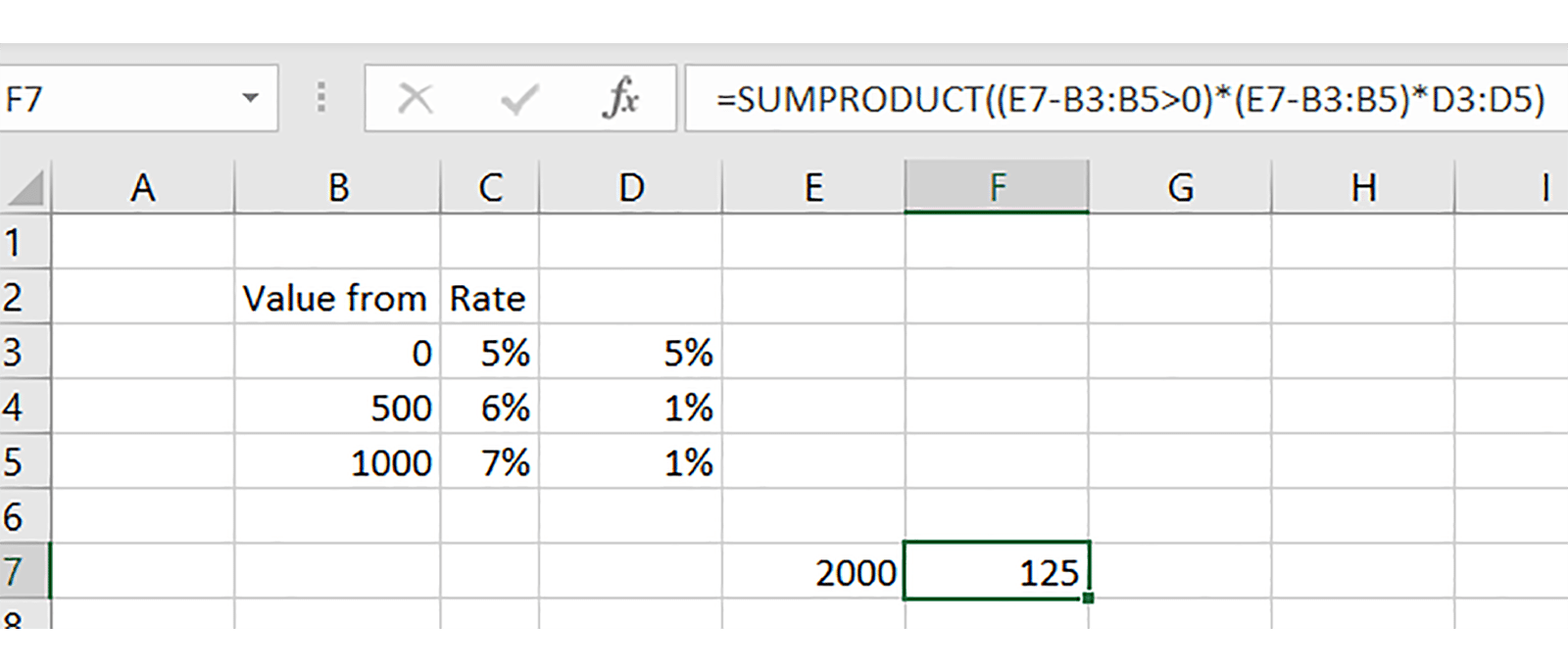
More detail in this TOTW.

How can I match partial data entry of two columns. ie. two sales persons using spreadsheet to record leads and I need to see if there's any duplication based on the trading names. The trading names may have spaces between words, or just incomplete entry. I'd like the spreadsheet to automatically highlight the suspected duplication.

This kind of partial matching, technically called “fuzzy matching”, isn’t really practical in Excel.

In pivot tables my table usually reverts to 'count' of values as opposed to sum of values. How can you make the default be sum?

The default is SUM if the column is all numbers; it defaults to COUNT if there is a mix of numbers and other values. Try checking that the columns you’re using are all numbers.

More and more websites are providing APIs with authorisation keys, is there a simple way that excel can pull the data in from these APIs into organised data fields?

What's the best way to connect Excel to accounting software? (e.g. Sage)?

If I receive a report on say a weekly basis, how can I compare easily from week to week any changes that are being reported?

All of these might be possible using Power Query, depending on the specifics. We have several PQ webinars in our archive at www.icaew.com/excelwebinars.

Is there a formula that can create a unique list of values from 2 different columns into one column?

In Office 365 you have the UNIQUE function; in older versions you would need to copy the data elsewhere and then use Data => Remove Duplicates.

With auto-filters you can pick “contain” as a condition e.g. has the word dividend in lots of words within a cell. Is there a way of writing a formula with either index and match or If statements to do this?

You can use an asterisk as a “wildcard” in a function like SUMIFS:

=SUMIFS(column of values, column of labels, “*dividend*”)

Is there any way of Unhiding a group of worksheets in a workbook?

In Office 365 you can select multiple sheets to unhide – at long last! – but in earlier versions you could use a macro such as:

Sub UnhideAllSheets()

Dim ws As Worksheet

For Each ws In ActiveWorkbook.Worksheets
  ws.Visible = xlSheetVisible
Next ws

End Sub

Is there a function or approach to take in Excel to highlight anomalies in data?

Is there functionality or any suggested approaches you would recommend be applied in identifying anomalies in large datasets for audit sampling purposes? (Criteria permitting)

There are a lot of options for investigating data using statistics and more – but it’s mostly going to be down to you to decide the approach you want to take and what kind of tests you want to perform to find outliers.

Is this being recorded? I would like to refer back to some items in my own time, as it's difficult to make notes.

Yes, this and many other webinar recording are available at www.icaew.com/excelwebinars.

SUMIF – How do you sum a number of figures in a column which matches the criteria rather than just the first figure in the column. I.e. In a cashflow, sum a number of cost categories to return a total for a particular month. At the moment I have to insert a SUMIF for each individual row Even if they are next to each other. Not so bad for 3 or 4 lines but impossible for many lines.

The easiest solution is to make a new column that sums those columns first, and then use that in your SUMIF.

Is there a way to remove the total in the legend of a waterfall chart? I use them to show variances and there is always an increase and a decrease but excel always adds a total and a colour for the total but this creates confusion as it is not shown on the chart.

Not sure how you’re using the Waterfall chart type, it should look something like this:

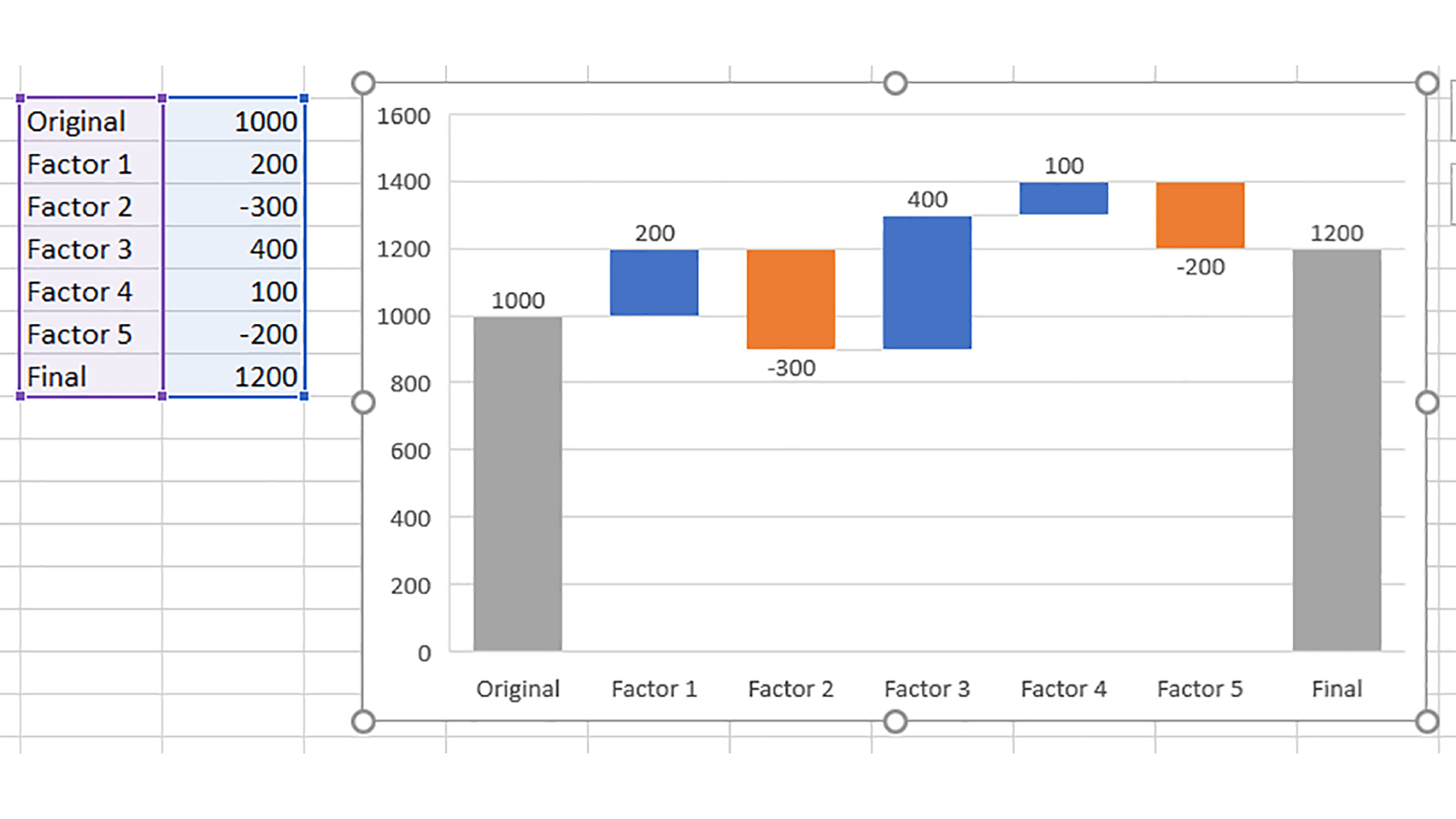
The key is to mark your original and final values as Total value types.

Can you make the index match find the second value?

If there is a second value, what you’re doing is something that any lookup function is appropriate for – these are all for situations with unique identifiers.

In a PivotTable, how do you get row labels side by side not above/ below each each other?

Design => Report Layout => Tabular.

Can you show how to add fields and items in pivots?

Please can you explain how to use formulas in pivot tables?

A calculated field is essentially an imaginary extra column that you can add in to your PivotTable. They can be created from PivotTable Analyze => Fields, Items & Sets => Calculated Field, and can then be defined by making a formula with the other column headings.

How do you add a quarterly interest charge in a formula that only picks up in the date referred to the month (the date in the cashflow runs over 5 years and therefore includes the year as well as the date)?

It sounds like you need to use an IF with a MONTH and MOD element, e.g.:

=IF(MOD(MONTH(date cell), 3) = 0, interest calculation, 0)

We have a macro which filters and unfilters a massive spreadsheet. But when new lines are added the macro needs changing to add the new lines to it. Is there an automatic way of doing this?

If the data were in an Excel Table instead, then the filter operation would apply to the whole Table if the macro were written appropriately. Or the macro could include code to identify the full range before applying the filtering.

If a SUMIFS function returns a result of zero but you know it shouldn't, what are common causes of this error to look out for?

The most common are either rogue spaces (e.g. “Hanover” vs. “Hanover “), or numbers that are formatted as text.

Re data source range I just use columns e.d. A:H so don't need to worry about adding extra rows - any problem with doing this?

It takes a bit more memory / processing, but for most workbooks the difference won’t be noticeable.

Do some formulas increase the size of workbooks more than others?

Yes, and have a particular impact on speed. Complex formulas like SUMIFS can make a difference if there are a lot of them, as can calculation-intensive functions like data tables. Calculation speed is also slowed down by volatile functions like TODAY, RAND, or INDIRECT, that Excel has to recalculate every time something changes.

Did you say there was a recording of this?

I did! All our webinar recordings are at www.icaew.com/excelwebinars.

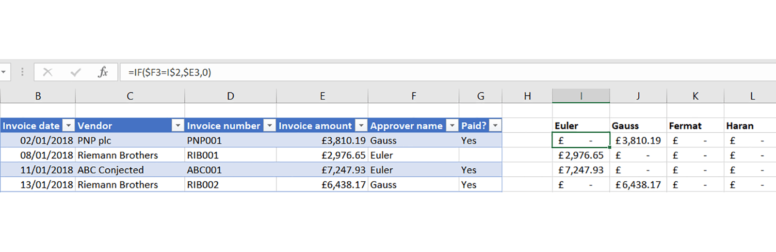
I have a data set that have by month, by company, by car make, by car model and by region. I am looking to plot say, 1) monthly Tesla Model 3 in China, 2) monthly Tesla sales all models in China, 3) Volkswagen Golf in China, 4) VW all models in China, 5) ...  If I want to plot all these hundreds of charts, what is the best way? I have tried 1)1) power queries but I have to duplicate the data, 2) pivot table but each time I need to change pivot table each time, 3) Filter but again very slow.  Is there any other ways? What is the best way please?

You can’t 100% do this easily, but there are some shortcuts.

First, to automate making a Pivot tab for each country/car combination, add a column to your data that concatenates these two into one, e.g.:

=Country column & “-” & Manufacturer column

Set up your PivotTable so that this is a Report Filter, then use PivotTable Analyze => Options => Show Report Filter Pages. This will automatically create a sheet for each value in the new column where that value is selected in the Filter, and name the Sheet accordingly. From here a macro could add a chart to each tab (only the Pivot will be copied automatically).

Would you please demonstrate using a chart linked to a pivot table?

You can add one from PivotTable Analyze tab – they work just like regular charts, except they automatically bring in new data as it is added to the Pivot.

If you have a table that has been subtotalled, how do you "copy" the subtotals to another worksheet (without it giving all of the rows). I currently go in and out of Word (copy to Word and then copy back to Excel) which seems mad.

If you press Alt ; when selecting data, only the visible cells will be selected, which lets you copy only the subtotals without copying the data in between them, once the rows are hidden with the group handles at the left.

Is it possible to have a running total as a column in a pivot table?

Yes – add the value to the Pivot, then select it in the Values area and go to Value Field Settings. Go to “Show Values As” and select “Running total in”, and then select the appropriate row label (usually the time series).

As pre course learning for the data analytics course I have to do a PivotTable course on Datacamp. I have started the course but am confused that it is using Google Sheets. How similar is the

Google software to Excel that I normally use?

It’s very similar, with essentially all the same common functions and abilities, but a different interface and less functionality for automation and integration in some niche areas.

In a waterfall graph is there a template/method that enables you to show a split of value in one of the steps, i.e. if the step is revenue, can you split by type?

You would have to show each type as a separate movement, or use a stacked column chart as a workaround instead (which was the common way of doing waterfall charts before they were added to Excel).

How to you return the row number of the last value in a column when there are gaps of data (blank cells) in the column please?

It’s a bit messy, but this array function can do it:

=MAX(IF(A1:A100<>"",ROW(A1:A100),0))

On pre-Office 365 you need to enter this with Ctrl Shift Enter.

I use msquery to bring data to Excel; I have tried Power Query but it always loads a preview of all the tables initially which makes it unuseable when dealing with lots of data, is there any setting to stop PowerQuery loading a preview of all the data tables (I have tried turning on "fastload" option).

PQ will load a preview but you might want to try using the “From folder” option, which will let you load all the files in a folder in a single query.

There have been a few occasions where an empty or a worksheet with just a few data entries is over 1-2MB. I have cleared the formatting, deleted data from those empty cells, but it is still an extremely large worksheet.

It’s worth checking what Excel thinks is the last cell on each sheet by pressing Ctrl End. If it is way off, try clearing all the contents from the spare cells, then save, close, and reopen the workbook.

Cell formatting - If you have a drop-down option on a cell, can you get the row to change to a different colour when a particular drop-down option is selected (again, text)?

Yes – if your dropdown is in A1, make a custom conditional formatting rule such as:

=$A1=“Hello”

If you have 2 pivot tables side by side, is there an easy way to get them to filter on the same thing without selecting each dropdown separately?

When is a good time to use SLICERS with pivots?

Try inserting a Slicer from the PivotTable Analyze menu – it’s a sort of filter that lives in its own window. Then you can select the Slicer and use the special Slicer menu => Report Connections to connect that Slicer to multiple PivotTables.

How can I show dates in a pivot table row? Whenever I try it automatically defaults into years and quarters.

This is called grouping and is automatic in some versions of Excel. Right click the column and select Ungroup.

Can you colour code cells based on whether they have inputted hard data or a formula? By formula. To help with modelling controls

Yes – Use Home => Go To => Go To Special to select either all constants or all formulas, and format as appropriate.

I created a 12 month cash forecast with cash in and cash payments with many rows & with sub totals of income & expense categories. Have monthly cash forecast with lots of rows with subtotals & totals am adding actuals each month & creating variances analysed between temporary & perm & creating cumulative variance columns also. The spreadsheet is now large as I’m adding lots of columns can you advise on better way to organise this data as I go through the months.

It sounds like you might want to look at just making a simple table of the values, a dropdown to pick which values to display in a human-friendly format, and then create the subtotals and comparisons with formulas from there.

Will you provide the excel spreadsheet - to review at own speed?

Yes, it will be attached to the recording at www.icaew.com/excelwebinars.

This session was great, are there plans for this to be a regular event?

Yes – this is already our third time doing it and we have two more in the diary at www.icaew.com/techfacevents.