Dynamic Lookups

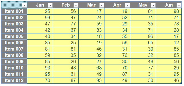
Imagine you had a dataset similar to the following:

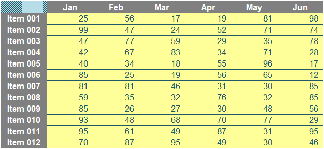
Your task is a simple one: for any given month and any given item, return the corresponding value (a so-called “two-way lookup”).  I shall ignore XLOOKUP as it’s not in all versions of Excel presently, so instead, I’ll use the functions INDEX and MATCH instead.  As a reminder:

INDEX

Essentially, INDEX(array, row_number, [column_number]) returns a value or the reference to a value from within a table or range (list).

For example, INDEX({7,8,9,10,11,12},3) returns the third item in the list {7,8,9,10,11,12}, i.e. 9.  This could have been a range: INDEX(A1:A10,5) gives the value in cell A5, etc.

INDEX can work in two dimensions as well (hence the column_number reference), e.g.

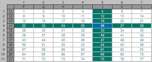
INDEX(F11:L21,4,5) returns the value in the fourth row, fifth column of the table array F11:L21 (clearly 26 in the above illustration). 

MATCH

MATCH(lookup_value, lookup_vector, [match_type]) returns the relative position of an item in a row or column vector that (approximately) matches a specified value.  It is not case sensitive.

The third argument, match_type, does not have to be entered, but for many situations, I strongly recommend that it is specified.  It allows one of three values:

• match_type 1 [default if omitted]: finds the largest value less than or equal to the lookup_value – but the lookup_vector must be in strict ascending order, limiting flexibility;
• match_type 0: probably the most useful setting, MATCH will find the position of the first value that matches lookup_value exactly.  The lookup_vector can have data in any order and even allows duplicates; and
• match type -1: finds the smallest value greater than or equal to the lookup_value – but the lookup_vector must be in strict descending order, again limiting flexibility.

When using MATCH, if there is no (approximate) match, #N/A is returned (this may also occur if data is not correctly sorted depending upon match_type).

MATCH is fairly straightforward to use:

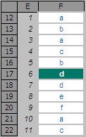
In the figure above, MATCH(“d”,F12:F22,0) gives a value of six [6], being the relative position of the first ‘d’ in the range.  Note that having match_type 0 here is important.  The data contains duplicates and is not sorted alphanumerically.  Consequently, match_types 1 and -1 would give the wrong answer: 7 and #N/A respectively.

INDEX MATCH

Whilst useful functions in their own right, combined they form a highly versatile partnership.  Consider the following common situation:

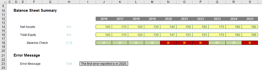
MATCH(1,$J$18:$S$18,0) equals five [5], i.e. the first period the balance sheet does not balance in is Period 5.  But we can do better than that.

INDEX($J$12:$S$12,5) equals 2020, so combining the two functions:

INDEX($J$12:$S$12,MATCH(1,$J$18:$S$18,0))

equals 2020 in one step.  Note how flexible this combination really is.  We do not need to specify an order for the lookup range, we can have duplicates and the value to be returned does not have to be in a row / column below / to the right of the lookup range (indeed, it can be in another workbook never mind another worksheet!).

However, this approach considers one criterion only (in the above example, ascertaining when the first misbalance occurs).  What happens if there is more than one criteria?  This can depend upon how the data is presented.

Consider pivoted data, i.e. where data is understood by cross-referencing criteria in two or more dimensions; in essence, the output is similar to results produced by a PivotTable.  For example, consider the following illustration:

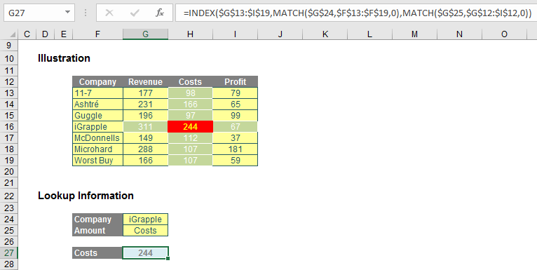
In this example, I have constructed a formula to determine the costs for iGrapple, a new company probably in the throes of lots of copyright infringement battles if it really existed.  The formula here uses INDEX(MATCH, MATCH) syntax, as it identifies the relevant row and column of the table to return.

The formula

=INDEX($G$13:$I$19,MATCH($G$24,$F$13:$F$19,0),MATCH($G$25,$G$12:$I$12,0))

considers the range $G$13:$I$19 and selects the row based on the result of MATCH($G$24,$F$13:$F$19,0), which identifies which row iGrapple is in the range $F$13:$F$19,  Further, the final argument selects the column based on MATCH($G$25,$G$12:$I$12,0), i.e. which column ‘Costs’ is in, in the range $G$12:$I$12.

The intersection of the row and column selected returns the pivoted value.

Returning to Our Scenario

Therefore, in our situation,

to determine a value, we would simply use the generic formula

=INDEX(Table_Data, MATCH(Item, Item_List, 0), MATCH(Month, Month_List, 0))

But what if the number of rows and columns were to extend?  Table_Data (the array of input cell values), Item_List (the vertical list of items in grey) and Month_List (the horizontal list of months in grey) would all be of variable size.  It’s not just the ranges that need extending; it’s the idea too.

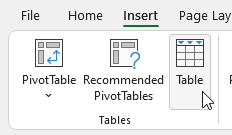
Whenever we have extendable ranges, we should use a Table (note: this is a proper noun).  I highlight the table and go to Insert -> Table (CTRL + T):

This calls the ‘Create Table’ dialog:

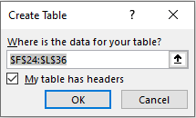
Ensuring you have checked ‘My table has headers’, our table (lower case “t”) is converted into a Table (upper case “t”).  All this work has made me thirsty: I think it might be time for some “t”.

Having had my t-break, the Table looks slightly different, viz

Four things have changed (only two of which are visible):

1. Filter dropdowns have been added to the first row. We don’t require these, so these may be removed by highlighting the Table and clicking on the ‘Filter’ button in the ‘Sort & Filter’ section of the Data tab on the Ribbon (ALT + A + T)
2. The top left hand cell has had text added, which defaults to the highly imaginative “Column1”. This is because all columns (fields) in a Table must be named and contain text not formulae.  This must not be deleted, but it will remain invisible in my example due to the formatting prevalent in this cell
3. Alternate rows are shaded differently.  Again, this is not noticeable, as I have already included my own formatting which overwrites this formatting. If my formatting were to be removed (e.g. change the cell style to ‘Normal’, i.e. Home -> Styles -> Normal), this shading would become apparent
4. In the very right-hand corner, a green, irregular hexagon is visible, which highlights the fact the Table may be extended both to the right and downwards, i.e. we have a range that may be extended.

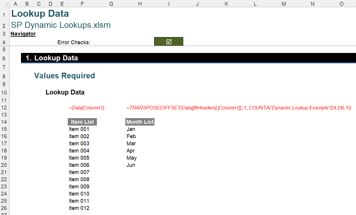
I now name this Table ‘Data’ (simply name it in the ‘Table Name:’ section of the ‘Properties’ group on the ‘Table Design’ tab of the Ribbon). Then, on a separate sheet I will call ‘Lookup Data’, I have created two formulae:

Just a minute!  I have stated I won’t use XLOOKUP because it’s not in all versions of Excel and then I quite merrily use dynamic arrays which are even less prevalent in Excel.

Er, yes.

You see, what I am not doing here is not essential and dynamic arrays will not be used to generate the formulaic solution.  However, creating these lists demonstrates the key concept I shall use to construct my formula.  Allow me to explain.

To generate the Item List (column F, above), I have simply used the formula

=Data[Column1]

This is quite simply the contents of the Column1 field in our Data Table.  I created the calculation simply by highlighting the contents (e.g. Items 001 to 012 in our example).  Generating a columnar list is simple; unfortunately, row lists are trickier – and this is where my second formula in column H comes in:

=TRANSPOSE(OFFSET(Data[[#Headers],[Column1]],,1,,
COUNTA('Dynamic Lookup Example'!24:24)-1))

TRANSPOSE and COUNTA are fairly simple to explain:

• TRANSPOSE does what it says on the tin: it swaps rows and columns around, so that rows become columns and vice versa
• COUNTA counts the number of non-blank cells in a range.  Therefore,
  
  COUNTA('Dynamic Lookup Example'!24:24)-1
  
  counts the number of blank cells in row 24 (which is the row containing the Table headings in my example) and subtracts one [1], so that the effect of the required text in the first column of the Table (Column1) is ignored.  This presupposes there is no other text, value or formula on this row.

The third function, OFFSET, perhaps needs a little more explanation.

OFFSET Reminder

OFFSET employs the following syntax:

OFFSET(Reference, Rows, Columns, [Height], [Width])

The arguments in square brackets (Height and Width) can be omitted from the formula – but they will prove to be useful in this article. 

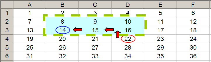
Most commonly, OFFSET(Reference, Rows, Columns) is employed to select a reference Rows rows down (-Rows would be Rows rows up) and Columns columns to the right (-Columns would be Columns columns to the left) of the Reference.  For example, consider the following grid:

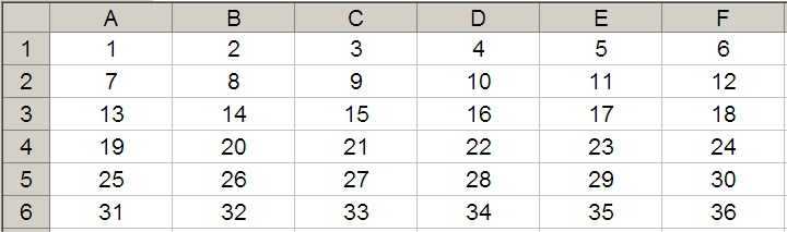
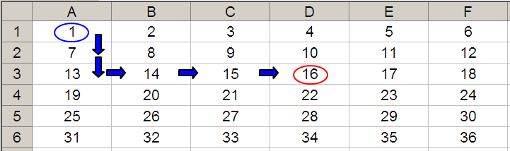
OFFSET(A1,2,3) would take us two rows down and three columns across to cell D3. Therefore, OFFSET(A1,2,3) = 16, viz.

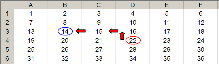
OFFSET(D4,-1,-2) would take us one row up and two rows to the left to cell B3. Therefore, OFFSET(D4,-1,-2) = 14, viz.

Let’s now extend the formula to OFFSET(D4,-1,-2,-2,3).  It would again take us to cell B3 but then we would select a range based on the Height and Width parameters.  The Height would be two rows going up the sheet, with row 3 as the base (i.e. rows 2 and 3), and the Width would be three columns going from left to right, with column B as the base (i.e. columns B, C and D). 

Hence OFFSET(D4,-1,-2,-2,3) would select the range B2:D3, viz.

Note that OFFSET(D4,-1,-2,-2,3) = #VALUE! in some versions of Excel which do not support dynamic arrays, since in these versions Excel cannot display a matrix in one cell, but it does still recognise it.  This can be seen as follows:

• SUM(OFFSET(D4,-1,-2,-2,3)) = 72 (i.e. SUM(B2:D3))
• AVERAGE(OFFSET(D4,-1,-2,-2,3)) = 12 (i.e. AVERAGE(B2:D3)).

Returning to Our Scenario (Again)

Now that our functions are understood, the second formula,

=TRANSPOSE(OFFSET(Data[[#Headers],[Column1]],,1,,
COUNTA('Dynamic Lookup Example'!24:24)-1))

is easier to follow.  The element

OFFSET(Data[[#Headers],[Column1]],,1)

returns the cell one column to the right of the Column1 header (i.e. Jan).  I have used this expression as the first column will always be consistently identified as Column1, but it’s possible for all other headers to be renamed.

The extension of this formula

OFFSET(Data[[#Headers],[Column1]],,1,,COUNTA('Dynamic Lookup Example'!24:24)-1)

creates a range starting with the second column header (Jan) and extending it to be COUNTA('Dynamic Lookup Example'!24:24)-1 columns across, i.e. it will be of the precise width of the non-blank range excluding the first column (Column1).

This is then wrapped in TRANSPOSE:

=TRANSPOSE(OFFSET(Data[[#Headers],[Column1]],,1,,
COUNTA('Dynamic Lookup Example'!24:24)-1))

Since the OFFSET formula is containing a row range, the result will be expressed across a row; using TRANSPOSE propagates this result down a column instead.

Since these two ranges are dynamic arrays, for versions of Excel that support dynamic arrays, these ranges may be referred to using the formulae =F15# and =H15# respectively (as # is the spill operator in dynamic Excel) and these references may be used to create data validation lists, should you wish.

However, if you don’t have dynamic arrays, keep reading.  It’s a “nice to have”, not an essential, element of the solution.

The dynamic lookup formula is “easy” from here:

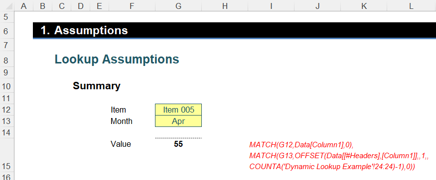
=OFFSET(Data[[#Headers],[Column1]],
MATCH(G12,Data[Column1],0),
MATCH(G13,OFFSET(Data[[#Headers],[Column1]],,1,,
COUNTA('Dynamic Lookup Example'!24:24)-1),0))

Rather than use the INDEX(MATCH, MATCH) approach detailed earlier, I use OFFSET(MATCH, MATCH), with the base cell being the first column header, Data[[#Headers],[Column1]], which is simply the structured reference for Column1 (cell F24 in our example file).  The two MATCH computations simply use the two lists generated earlier to find the correct row and column displacements.

Please refer to the attached Excel file for a modelled example.

Word to the Wise

This is another common problem in Excel.  All too frequently, modellers forget to put the reference table in an Excel Table.  For those that manage this, many are unsure how to reference a row dynamically.  The OFFSET(COUNTA) approach has been available for many years, but few ever utilise this function combination.

Try it out!