How to review a spreadsheet: Part 2 - data review

Data specification

When a spreadsheet is built, the author will have written formulae based upon their view of the source data. However, ambiguity for users can be created by the following:

Sign - should the data be entered as a positive or negative value? For balance sheet data, the item of receivables (debtors) might be entered as a positive, but does that mean payables (creditors) should be entered as a negative? A helpful convention is to have all data entered as a positive and use formula to change sign where necessary.

Currency – when working with multi-currency spreadsheets make sure it is obvious which currency is being used for each of the sheets, but especially for each data input and the derived outputs.

Order of magnitude – is the data entered as an absolute number, in thousands, millions etc.

In designing an input area on a spreadsheet, it is helpful to have both a detailed description of the data item as well as a column defining the units for the inputs. The example below is the data for a restaurant model.

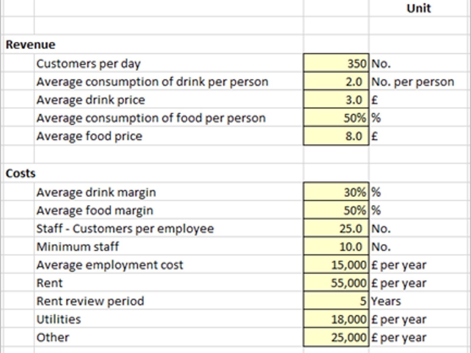
Data Source – it may also be helpful to note beside each item where the value has been sourced. This will help in any review to trace back to the information source and validate the numbers have been entered correctly.

Data validation

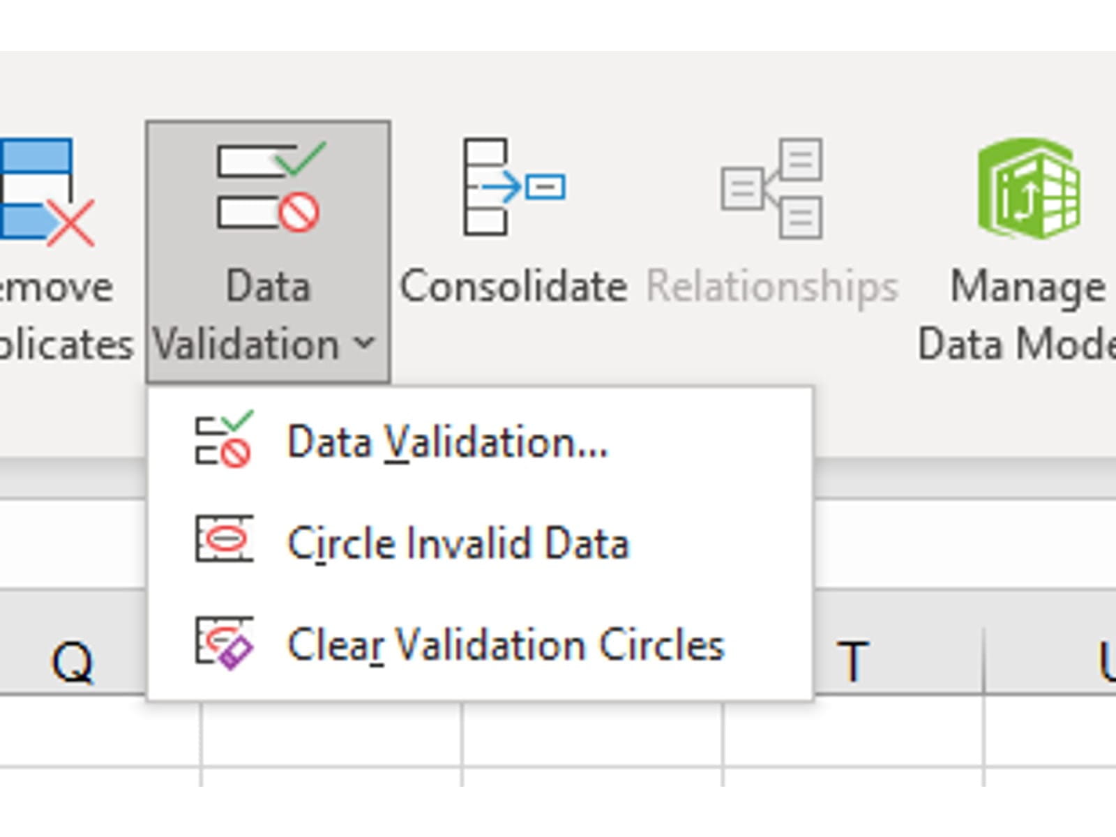
On the Data ribbon in the Data Tools section there is a drop down set of three Data Validation tools. Spreadsheet builders should be encouraged to use these functions to assist in ensuring valid data is being entered.

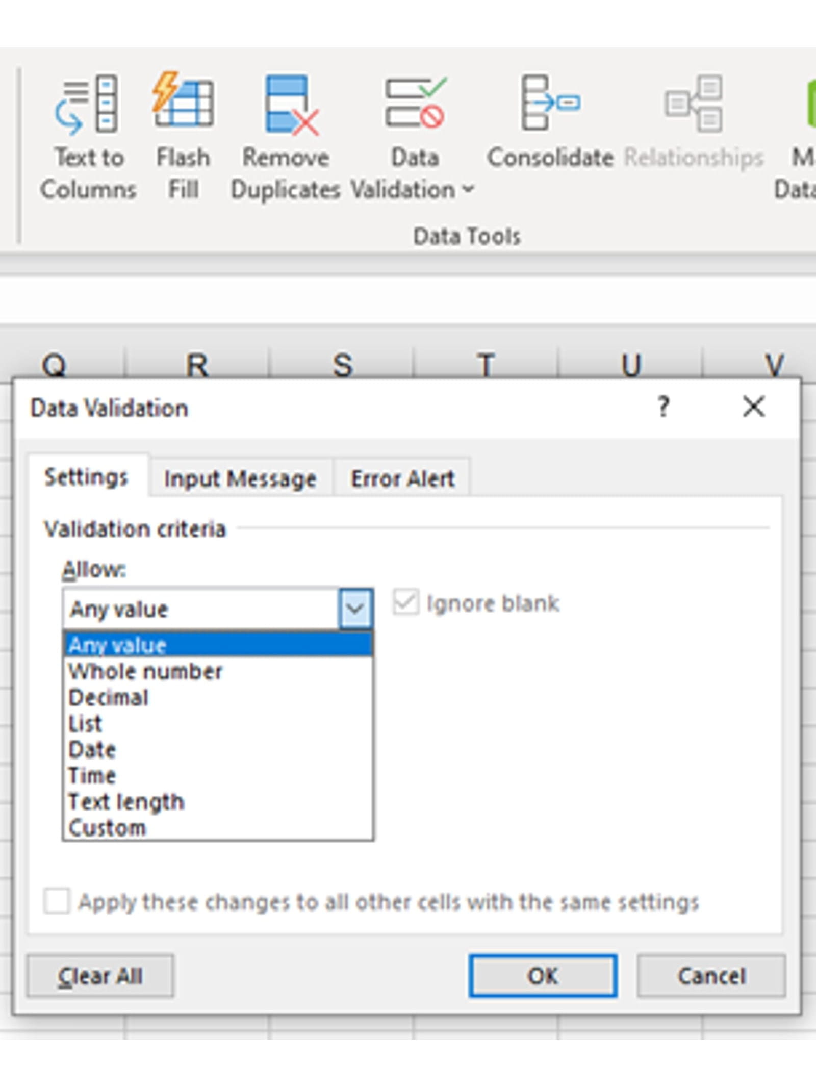
From the drop down at the top of the Data Validation dialog box you can see 8 categories that can be defined. The date, time and text options will ensure the correct data type is entered in a cell.

The most common uses are the numerical options where the valid input range can be linked to cell values. Thus, this tool can be used across a whole block of inputs very quickly rather than setting up each input individually.

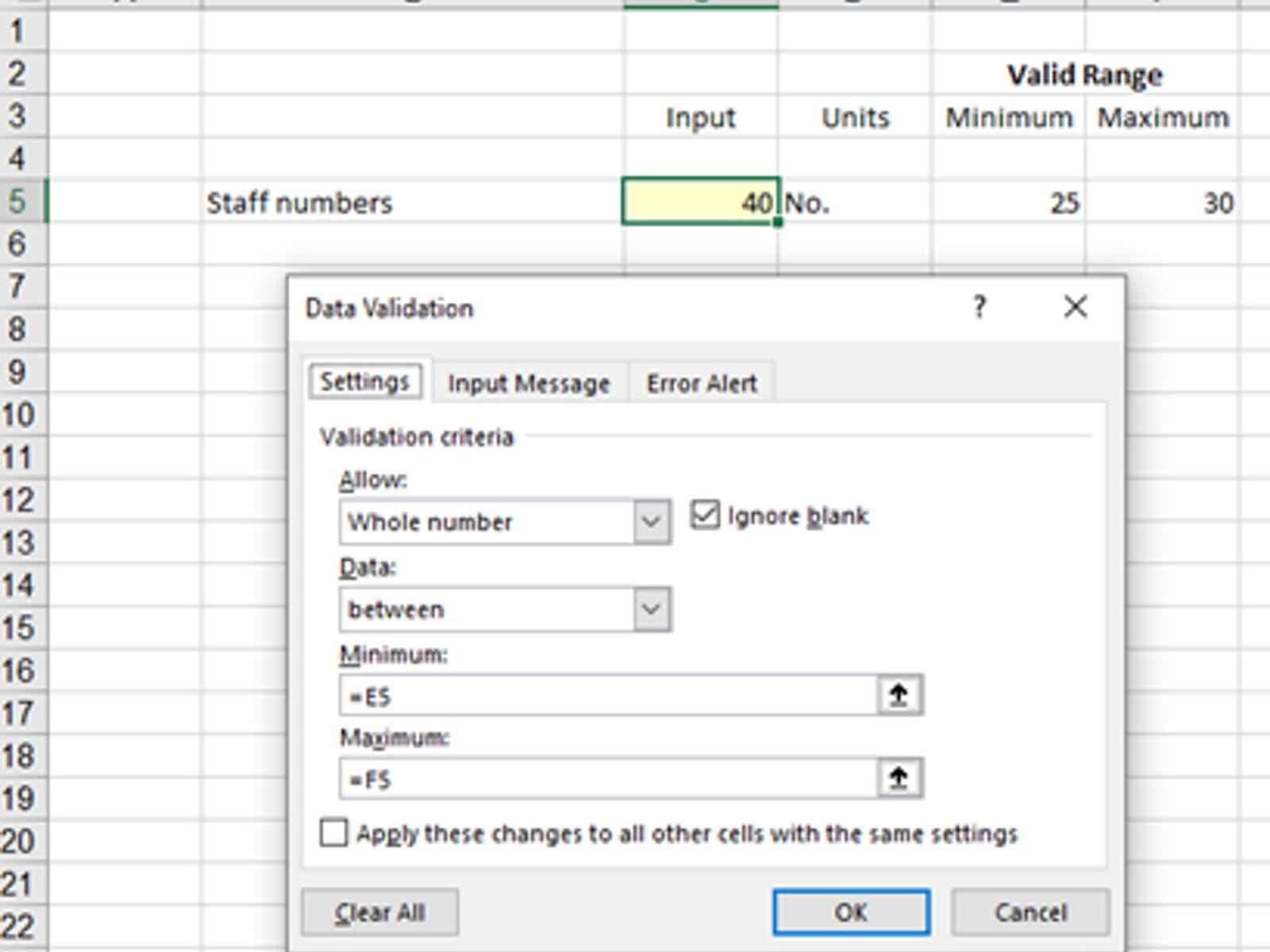
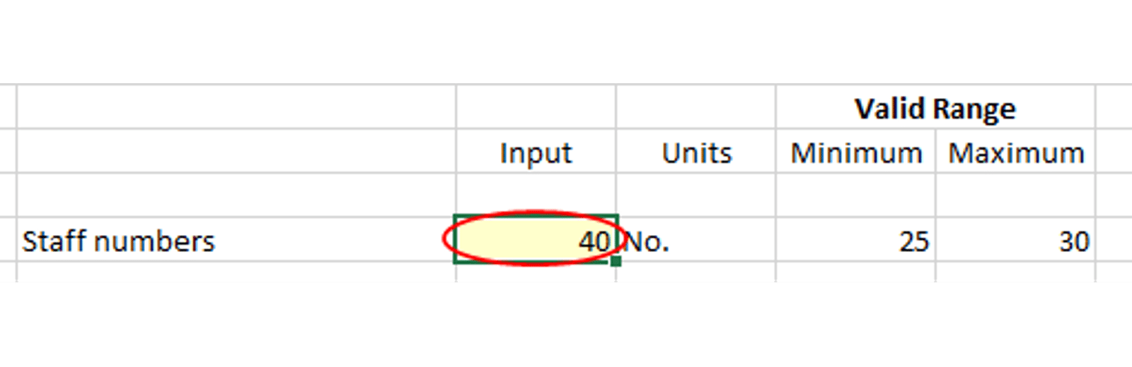
In the above example the input cell is C5 and the valid range is defined in E5 and F5. Using this style not only makes the valid range visible to the user but also allows the cell validation criteria to copied down a whole column of inputs and set up for an entire range. NB it may be appropriate to protect the maximum and minimum cell ranges to avoid them being changed by users.

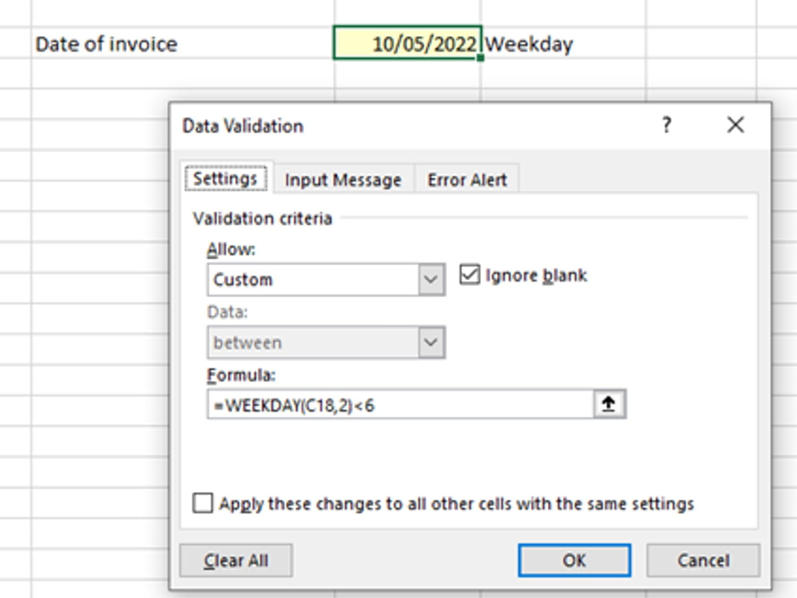
At the bottom of the list of 8 validation criteria is Custom. This option can be used to set up an Excel Formula where the result is True or False. True is used for data that is valid, False is for Error. For example, if you wanted to ensure that a date entered was a weekday and not a weekend you could use:

In the first data range example you will notice that the input value in C5 is outside the valid range. To highlight errors use the Circle Invalid Data option.

The result will look as follows:

The other two tabs on the Data Validation dialog box provide the options to script your own Input Message and style of Error Alert. Unhelpfully the text script used for the Input Message cannot be linked to a cell values. Eg it might be helpful to have the valid data range in the Input Message, but this can only be typed not cell linked.

When reviewing a spreadsheet the first part of a data review is to check the source of all data values are correct, make sure the values fall within valid ranges and where Data Validation has been used the option of Circle Invalid Data has been selected and any errors identified.

Test data

To check that the spreadsheet functionality is working effectively it can be helpful to have a set of test data where the result is known. However, this may not always be practicable as the result may only be known by building the spreadsheet…. Therefore, an effective alternative is to build component parts where the answers can be determined and known.

For example, revenue might be derived from customers x units x price. This calculation can be checked that it matches with the value showing in the spreadsheet. By breaking down the spreadsheet into sections and checking that a subset of data gives the correct results can ensure the validity of components.

Beware of relying upon only one set of data. It is better to run the with two sets of test data. For example, if there was a hard coded number for price that had been buried in formula, it might be valid for one set of data, but would only show up when the second send of data failed.

Zero inputs

Logic might suggest that if a data set of zeros is entered then the output should also be zero. This is very useful if it were true, however it is more likely to throw out a lot of errors especially #DIV/0! The benefit of clearing all the errors to ensure that zero in = zero out must be judged.

What you are aiming to find is the use of any hard coded numbers that may be hidden and corrupting the user seeing the true impact of flexing inputs. We will provide some additional help to identify hard coded numbers by using Go To Special in blog 6.

A way around having a #DIV/0! Error is to use the function =IFERROR(formula, value if error) and to set the value if error to 0. The danger of this function is that it may disguise a host of other errors (such as missing references #REF!, absent range names #NAME? etc.) that are then conveniently cleared to zero at the same time.

The way of trapping just a #DIV/0! Error is simply to do an =IF test on the denominator to see if it equals zero before the calculation is completed. While this is more time consuming to set up it may provide more confidence that other errors are not being masked.

Stress testing

This is the opposite of Zero inputs, it is where very large value for inputs are entered. This tests if error trapping is working to catch values for which the spreadsheet was not designed to handle.

In many ways it checks how well the Data Validation was set up, as explained at the start of the blog.

Delta testing

This is a way to sense check spreadsheet functionality more than data validation. It is where the results of two data sets are compared. The check here is whether the input changes between the two sets would be reasonably expected to generate the output changes.

For example, if you put prices up by 1%, but all other inputs remained the same – what happens? Clearly revenue should go up by 1%, but as volumes have not changed the costs should remain the same. 

The process involves looking at input values either in isolation or in small sets. Changing too many inputs at once makes the evaluation of what has changed too complex to interpret.

With a robust set of input data, it is now down to the formulae to generate valid results. In blog 3 we will look at completing Analytical Reviews to provide signals that the outputs are looking valid. These will be a mixture of visual clues (charting) and calculated clues (ratios).