
Time for a running commentary on multiple running totals.
You have to be careful calculating cumulative balances (“running totals”) in Excel, as they can be harder to construct than you might think initially. Consider the following table:
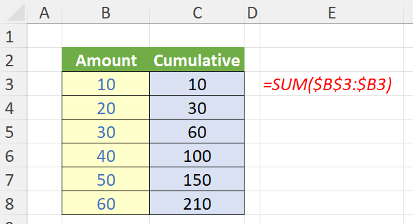
Ensuring you anchor your cell references correctly (either by typing in the ‘$’ or by using the F4 function key in ‘Edit’ [F2] mode), the formula
| =SUM($B$3:$B3) |
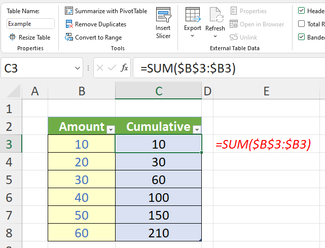
in cell C3 will achieve the desired effect. However, things are a little more “fun” if we turn the range into a Table using CTRL + T, and calling the resulting Table ‘Example’ (say):
Adding a row is interesting:
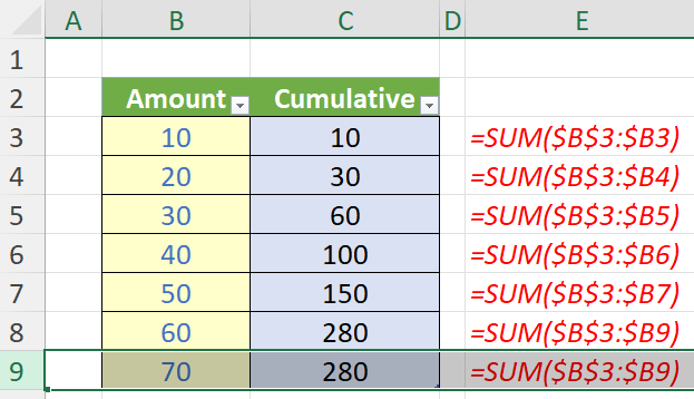
Oops. An alternative formula seems to solve this problem:
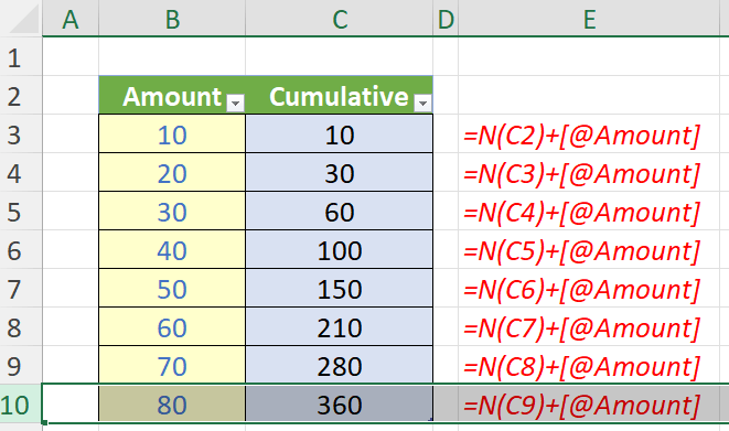
Note the revised formula in cell C3:
| =N(C2)+[@Amount] |
This is a mixture of Excel cell referencing (e.g. C2) and Table (or “structured”) referencing (e.g. [@Amount], meaning the Amount value on that row). The N function takes the numerical value of the cell referenced, i.e. text is treated as having zero value, rather than causing a #VALUE! error if used in a summation otherwise.
Unfortunately, this alternative doesn’t work in all situations either. To break it, simply insert a row into the table:
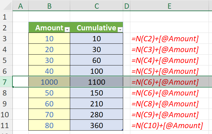
Tables and running totals do not seem to mix, so bear this in mind. It’s simpler just to use standard tables, as in the first screenshot (above).
But let’s complicate things further. Imagine you have a data table you collate daily regarding inventory movements, viz.
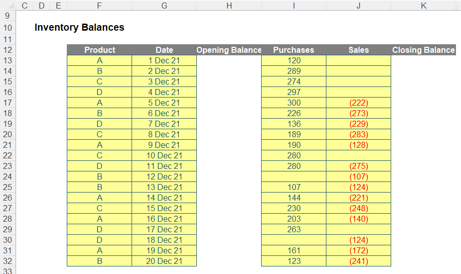
Here, I have several different inventory items that are collated on a daily basis in a table (lower case “t” – not an Excel Table, based upon my observations above). I can assume column G will keep dates in ascending order, i.e. that dates will either increase or be equal to the previous row’s date.
I want to keep a running total of the opening and closing balances, leaving the format alone (I might be using the table as the source for a PivotTable, for instance). The question is, how do I do this?
The Closing Balance formula (column K) is simple enough:
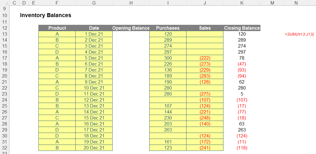
The formula in cell K13, for instance, is given by
| =SUM(H13:J13) |
The issue is clear: how do you calculate the opening balances? They aren’t necessarily the closing values from the row above. We need to find the last occurrence of a purchase or sale for that product. If the products were sorted, we could use the LOOKUP function, as this finds the last occurrence of sorted data. Unfortunately, that will not work here.
Therefore, we need to find the last date for that product, and then look up the Closing Balance on that date for that product. Assuming the fact we might have two or more records for the same product on the same date, we cannot use SUMIFS: we will need to use a “helper” column instead, in order to look up the last occurrence of a given date / product combination.
The Helper field is easy:
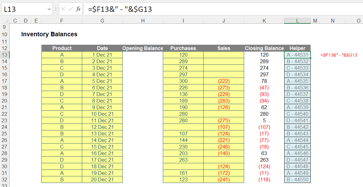
The formula in cell L13 is given by
| =$F13&" - "&$G13 |
Notice the use of a delimiter. The “ – " separates the product and the date so that there can be no confusion. Further, the date appears in its serial number form, i.e. counting the number of days where 1 January 1900 is Day 1 etc. (and forgetting that 1900 wasn’t a leap year, but that’s a story for another day!).
Now that we have our Helper column, the formula for the Opening Balance (column H) can be created:
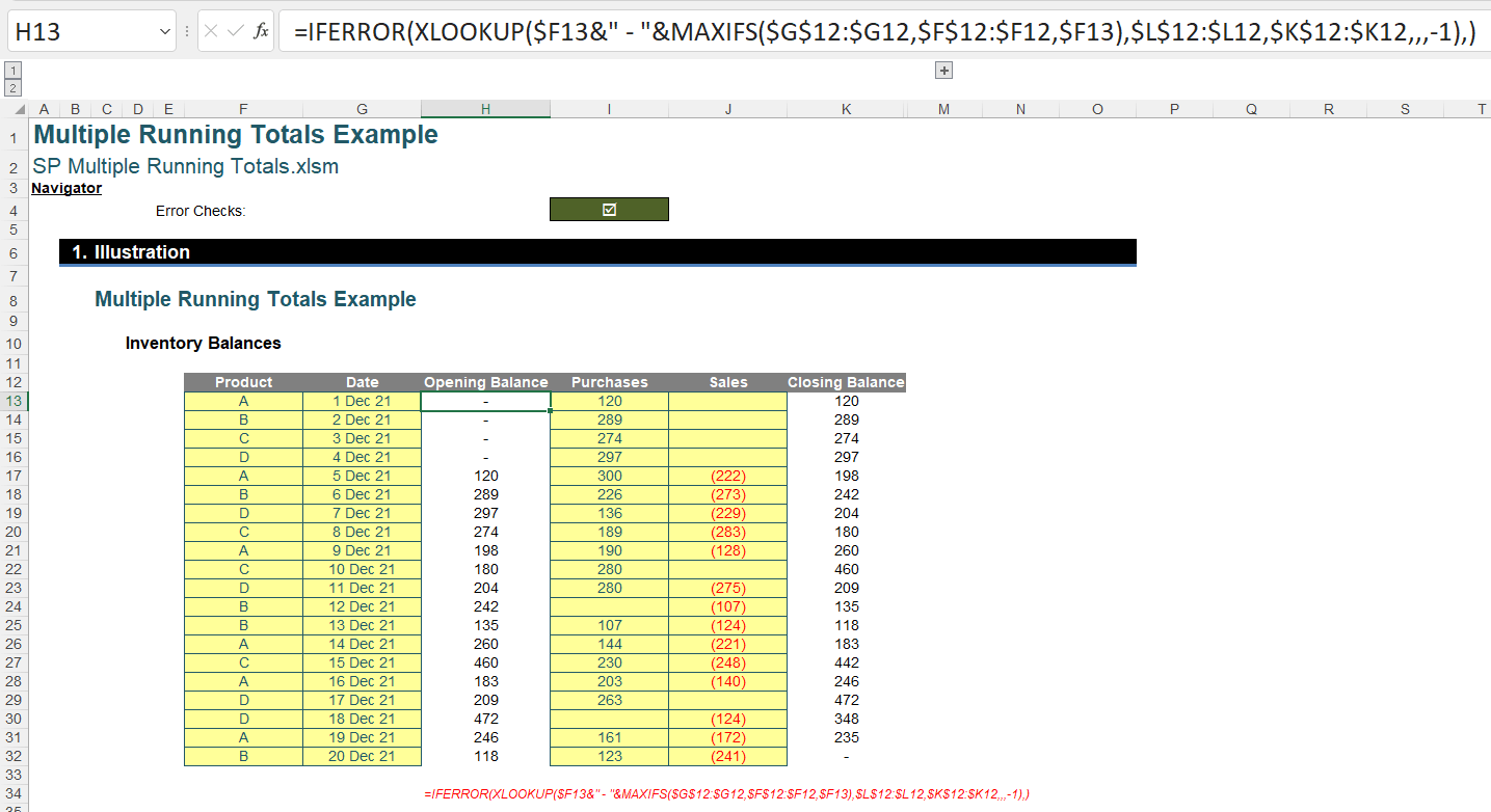
The formula in cell H13 is given by
| =IFERROR(XLOOKUP($F14&" - "&MAXIFS($G$12:$G13,$F$12:$F13,$F14),$L$12:$L13,$K$12:$K13,,,-1),) |
It may seem a monster of a calculation, but it’s not so bad once you split it into its calculable components.
The core calculation
| MAXIFS($G$12:$G14,$F$12:$F14,$F15) |
uses the function MAXIFS to find the maximum value in the range $G$12:$G14 (i.e. all the dates for the rows preceding the current record) subject to the product in the range $F$12:$F14 (i.e. all the products for the rows preceding the current record) equalling the product in the current row / record (i.e. cell $F15). This maximum value is the last date the current product was recorded in the table.
This value is then concatenated with the product:
| $F16&" - "&MAXIFS($G$12:$G15,$F$12:$F15,$F16) |
This will then give a value that may be searched in the Helper column using XLOOKUP:
| XLOOKUP($F16&" - "&MAXIFS($G$12:$G15,$F$12:$F15,$F16),$L$12:$L15,$K$12:$K15,,,-1) |
The first argument is simply the concatenation created in the last step. This combined value is then sought in the Helper column in the range $L$12:$L15 (i.e. all the concatenated values for the rows preceding the current record) and the value returned is the corresponding Closing Balance in column K in the range $K$12:$K14 (i.e. all the Closing Balance amounts for the rows preceding the current record). The final term in the XLOOKUP function (-1) is cited to force XLOOKUP to search in reverse order, i.e. from the final row above to the first row above. This is to ensure the correct Closing Balance is obtained if two records cite the same product on the same day.
The final formula,
| =IFERROR(XLOOKUP($F14&" - "&MAXIFS($G$12:$G13,$F$12:$F13,$F14),$L$12:$L13,$K$12:$K13,,,-1),) |
simply wraps everything in an IFERROR statement so that zero [0] is returned should there be no occurrence of the product previously. Easy when you know how!
Please refer to the attached Excel file for a modelled example.
Word to the wise
This is a problem that was awkward to model before the advent of XLOOKUP and dynamic array formulae. This is because MAXIFS needs to be replaced by the array formula {MAX(IF)} (using CTRL + ALT + DEL), plus you have to employ an old LOOKUP trick to find the last occurrence of data in an unsorted list (given LOOKUP requires data to be sorted!).
I don’t go through it here, but it can be done:
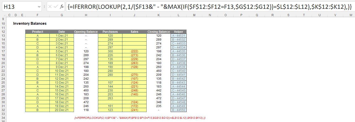
For example, the formula in cell H13 is now given by
| {=IFERROR(LOOKUP(2,1/($F13&" - "&MAX(IF($F$12:$F12=F13,$G$12:$G12))=$L$12:$L12),$K$12:$K12),)} |
It may seem to be of similar length, but the ideas behind this formula are more complex. I would definitely recommend the original solution mentioned, but I include this alternative in the attached Excel file.
