Isolating your inputs

Much of this post is applicable to all spreadsheets you might build. In fact this post is essentially the 10th of the ICAEW's Twenty Principles for Good Spreadsheet Practice (separate and clearly identify inputs, workings and outputs). But I have seen these simple tips transform chaos into order when it comes to monthly reporting.

Your Management Accounts Pack inevitably includes a number of cells that need to be edited. How many there are will depend on how well the spreadsheet is structured, and how much of the data is held in your accounting system (more on this next month).

Minimise the editing required

The first step is to edit the spreadsheet to minimise the number of cells that need editing each month-end.

The posts so far in this series have largely been focused on specific applications of this step - automating dates and text based upon entering the period number once (part I), removing the need to edit formulae pulling in comparative data (part II) and removing the need to edit charts (part III).

This principle should be extended to cover any other examples of where cells are required to be edited.

If you are editing formulae on any kind of regular basis in your management accounts pack, then this should be addressed first. Identify the elements of the formulae that are being edited and give those variables their own cells, which are then referenced by the formula, leaving the formula untouched each month.

Examples of the types of variables that might need to be stripped out of formulae like this are period number, any statistics (such as tonnage, units, etc,), no. of weeks in month, etc.

As stated in the 10th Principle: "Design to ensure that any input should be entered only once."

Gather all of these inputs together

Once you have minimised the number of inputs required, the next step is to bring them all together in one place.

It can be very time-taking and prone to error to go through the whole spreadsheet, remembering which cells need to be edited.

It is much better to clearly have all of the inputs in one place.

If you have large tables of inputs, maybe pasting in (or importing) a trial balance or maintaining a cross-reference table, then these can be given their own sheet. But these sheets should be grouped together, preferably all with the same colour tab, so that they can be easily seen as the input sheets.

The rest of the inputs should usually be gathered on one sheet. In some cases where there are a lot of inputs, you may want this to be two sheets - one for the regular changes and another for maintaining standing data that would rarely change. This approach helps to reduce clutter on the tab for the normal monthly changes.

Sometimes you may have a selection of inputs together and be tempted to leave them where they are. It is simple to bring these onto the Input sheet and it will pay to do so.

For example, let's say that on a 12 month P&L report, we enter tonnage sold at the top of each month. Simply add a row of 12 cells to the input sheet and reference the cells on the 12 month P&L to these cells. So we enter in the period 1 cell on the 12 month P&L

=Input!B5

and then copy this along the row (assuming the period 1 input is on cell B5 of the Input sheet).

If we don't want zeros to appear in the months we haven't entered yet, we could replace this with:

If (Input!B5="","",Input!B5)

Not only should all of these inputs be gathered together on one (or two) tabs, but it should be clear which cells are the input cells.

I usually do the following:

• Give the whole sheet a background colour
• For each input cell:
• Remove the background colour
• Unlock the cell (on the protection tab of the Format Cells dialog)
• Apply any data validation if appropriate

I then protect the sheet, un-ticking "Select locked cells" on the allow list (this means that the user cannot click in any cells other than the ones requiring input and can use the tab key to quickly move through the cells that do require input).

A typical Input sheet might look like this:

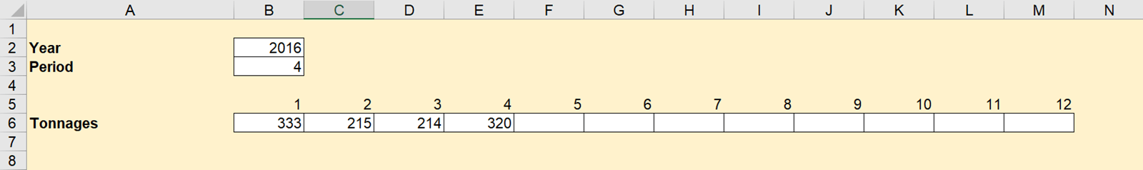
Following these simple steps means that each month, all you need to do is paste in or import the TB to its own tab and update the fields on the Input tab. There should be no requirement to edit anything else in the Management Accounts Pack (unless you have a narrative to write - which could also be entered on the Input tab and pulled into its appropriate place with a formula.

This approach can save a huge amount of time each month, and even more time when training a new member of staff to update the management accounts!

It also significantly reduces the risk of errors - you can see at a glance whether you've updated the fields that need updating.

In part V, we take a look at a better way of treating statistics such as the tonnages above, to even further reduce the editing required in the spreadsheet.