Ticks and crosses

I'm sometimes asked about the easiest way to insert ticks into Excel cells. I'm not sure that I've yet discovered the easiest way and would welcome any other suggestions.

Here are a few ideas.

Symbols

This is probably the most obvious method. You can use the Insert Ribbon tab, Symbol option to find a tick symbol to insert. As well as inserting the chosen character directly from the Symbol dialog, the dialog shows the ASCII number of the character that you have used. You can type this in using the keyboard as four characters with a leading zero if required, holding down the Alt key and using the numeric keypad. It is possible to use File, Options, Proofing, AutoCorrect to set up text that will automatically be replaced by the chosen symbol, but the keyboard shortcut and the AutoCorrect method both need the font to be changed to the correct one for the symbol (usually Wingdings).

Conditional formatting

A more colourful alternative is to add a conditional format to the cells that need to contain the ticks (and possibly crosses). To start with, we use the appropriate Icon set:

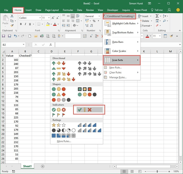
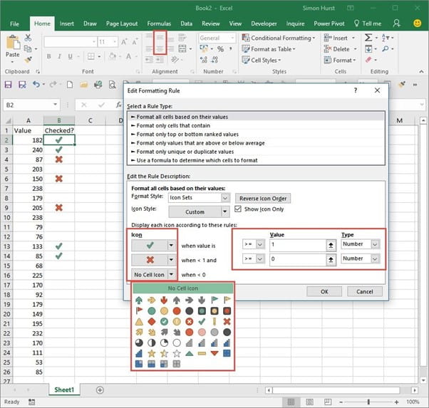
By default, Icon Set conditional formats will be based on looking at the values in a range of cells and allocating icons based on proportions according to how many icons are in the set. In our case, with three icons, icons are allocated to each 33% of values. We want our icons to work differently, so we use Manage Rules, Edit Rule to access the detailed options (note that Excel 2007 doesn't include the options to select icons separately):

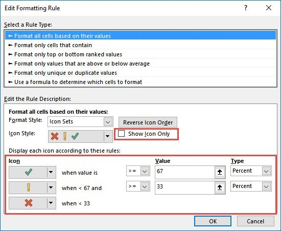
We only want to show the icon in the cell, so we turn on Show Icon Only. We just want to use the tick and the cross, so we choose the appropriate icon in each of the dropdowns – we could either set the bottom icon to 'No Cell Icon' or select an icon to display as a warning if a number less than 0 is entered. We have changed the Type to 'Number' for each of our icons and set the value for the tick to >=1 and for the cross to >=0. The remaining icon will be used for numeric values below zero. Text values will not be affected by the conditional format and will display as they have been typed. The user can now just enter 1 in the cells to which the conditional format has been applied to display a tick and 0 to display a cross. We have used the text alignment commands to centre the icon in the cell:

Google Sheets

If you're using Google Sheets instead, you can add tick boxes directly to cells from the 'Insert' menu. This makes it much easier to create checklists, with the added bonus that they are stored as binary true/false values, which means they can be interacted with in formulas too. This is touched on in Tip #461 as well as the webinar Excel vs Google Sheets.