
Many Excel features, methods and techniques are equally useful to any spreadsheet user. In this article, we focus on a topic of particular relevance to accountants and others working with financial data – number formats.
This article was originally published in 2019.
It has been reviewed for relevance to latest Excel developments and while some screenshots may reflect older versions of Excel, the functionality is unchanged.
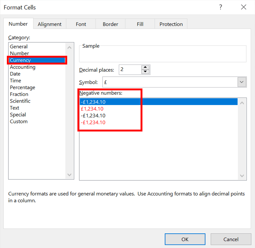
The Number format dropdown (in the Number group of the Home Ribbon tab) displays the different types of number formats that Excel can apply. Some of the built-in number formats depend on settings elsewhere in Windows. For example, these detailed options for Currency formats show negatives with a minus sign:
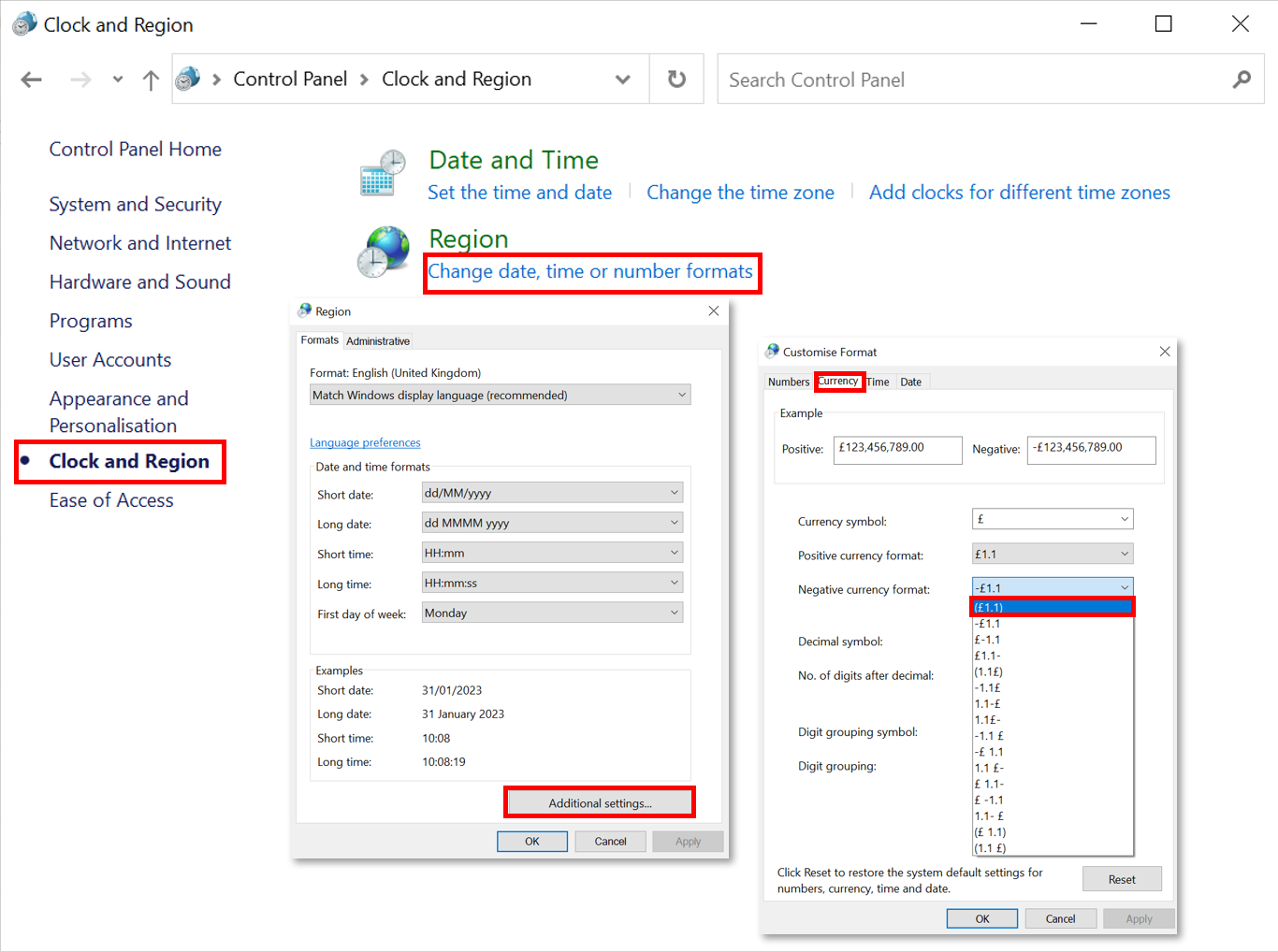
Here, we have delved down through many levels of Windows Region Settings to find the regional number formats and the Currency tab, where we have selected a Negative number format that uses brackets rather than a leading minus sign:
Having made this change, the Excel Currency number format options will now include negatives with brackets:
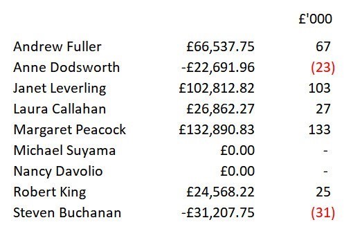
Alternatively, you can create a Custom number format to ensure the use of brackets rather than a minus sign. Using a Custom format also has the advantage of giving you control over other aspects of the number format, such as replacing a zero with a dash for a zero value.
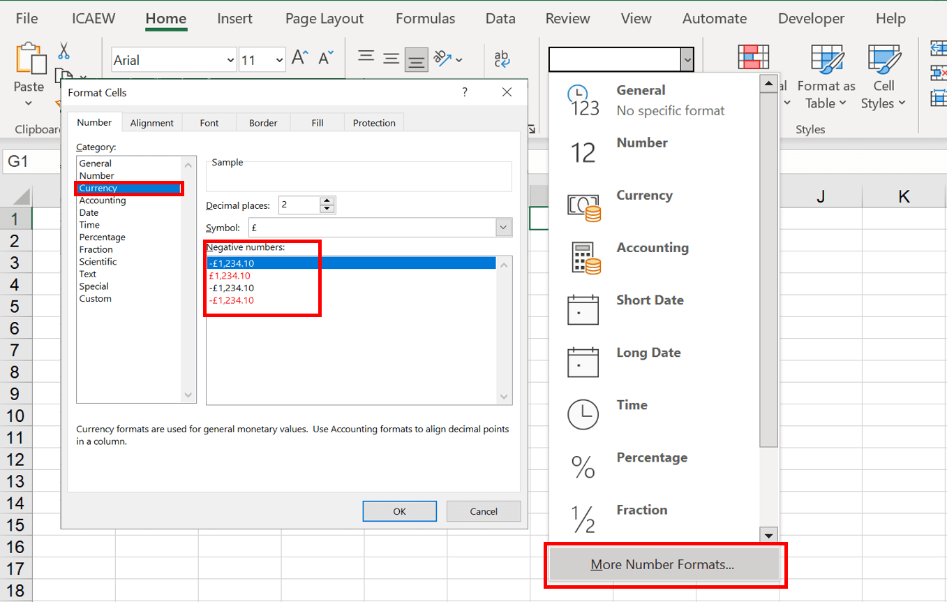
To access existing custom number formats and create new formats, select Custom (in the Number tab of the Format Cells dialog, shown above). This dialog can also be displayed by choosing Format Cells from the right-click menu, or by clicking the Number Format dialog button at the right-hand side of the Number group title in the ribbon.
A Custom number format can have up to four sections:
| Section | Use | Example | Result |
|---|---|---|---|
| 1 | How positive numbers are to be displayed | #,##0.00_) | This uses thousand separators and two decimal places. It also uses a space equal to the width of a closing bracket to the right of the number (to ensure that negative and positive numbers line up). |
| 2 | How negative numbers are to be displayed | [red](#,##0.00) | This shows negatives in red, with brackets and with thousand separators and two decimal places. |
| 3 | How zeros are to be displayed | -? | This displays a dash inset from the right by one space. |
| 4 | How text entries are to be displayed | @ | This displays whatever text is entered in the cell. If you include a text section without an entry, then the cell will not display text. This section is usually omitted altogether. |
For a typical accounting format (with brackets for negatives) the format could be:
#,##0.00_);[red](#,##0.00);-?
We'll look at each of the sections in more detail, including the various codes used within a custom number format:
Section 1 - positive numbers
#,##0
The hashes (#) will only display 'significant' digits - this means leading zeros will be suppressed. The 0 means display a zero in this position even if the number is less than 1.00. An example should make this clearer:
| Format | Value | Result |
|---|---|---|
| #,##0.00 | .98 | 0.98 |
| #,###.00 | .98 | .98 |
Finally, the comma makes Excel use the comma as the thousands separator.
Also note the use of the underscore. This causes Excel to leave a space equal to the width of the character that follows the underscore. In this example, we have used _) to include an amount of space at the end of a positive number equal to the width of a closing bracket. This ensures that negative and positive figures in the same column line up exactly.
Section 2 - negative numbers
[Red](#,##0)
In the second section there are a couple of additional elements:
The name of one of the eight main colours in square brackets causes the numbers to be displayed in that colour. In our case, negative numbers will be red. It is perfectly possible to apply colours to positive numbers as well, by preceding the first section with the colour in square brackets, e.g. [blue].
Brackets are used to ensure that negative figures are shown in brackets.
Section 3 - zero values
-?
We have entered a dash followed by a question mark. The question mark inserts a space in order to move the dash in one character from the right-hand edge of the cell.
Section 4 - text
This section is not used in our example. If you do not use this section, text will be displayed as it is entered. If the fourth section is blank, any text entered will not be displayed. The use of the 'at' character (@) will display any text as it is entered. You can also combine the text entered with some fixed text. For example:
#,##0_);(#,##0);;"Sales of "@
will display 'Sales of ' followed by the text entered into the cell. If a number is entered, just the number will be displayed, formatted as shown by the positive and negative sections.
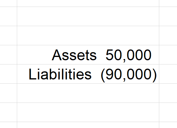
You can also include text as part of a number format. For example, if you want to label positives as 'Assets' and negatives as 'Liabilities', you could use the following custom format:
"Assets " #,##0_);"Liabilities " (#,##0)
This would give the results:
Asterisk
An asterisk followed by a character will fill the available space with repetitions of that character. In some of the built-in number formats, this is used to position the currency symbol at the left of the cell:
_(£* #,##0_);_(£* (#,##0);_(£* "-"_);_(@_)
Because the asterisk characters are followed by spaces, space characters will be repeated between the currency symbol and the first number or bracket, to 'push' the currency symbol to the left edge of the cell.
With this, we have covered the creation of our perfect number format.
Archive and Knowledge Base
This archive of Excel Community content from the ION platform will allow you to read the content of the articles but the functionality on the pages is limited. The ION search box, tags and navigation buttons on the archived pages will not work. Pages will load more slowly than a live website. You may be able to follow links to other articles but if this does not work, please return to the archive search. You can also search our Knowledge Base for access to all articles, new and archived, organised by topic.
