Useful Features of XLOOKUP

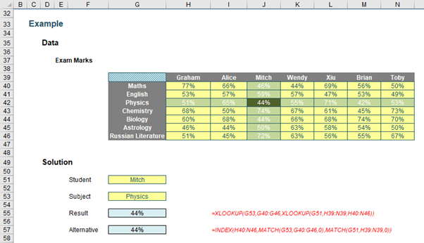
XLOOKUP can be used to perform a two-way match, similar to INDEX MATCH MATCH:

Many advanced users might use the formula 

=INDEX(H40:N46,MATCH(G53,G40:G46,0),MATCH(G51,H39:N39,0))

where:

• INDEX(array,  row_number, [column_number]) returns a value or the reference to a value from within a table or range (list) citing the row_number and the column_number
• MATCH(lookup_value, lookup_vector, [match_type]) returns the relative position of an item in an array that (approximately) matches a specified value. It’s most commonly used with match_type zero (0), which requires an exact match.

Therefore, this formula finds the position in the row for the student and the position in the column of the subject. The intersection of these two provides the required result.

XLOOKUP does it differently:

=XLOOKUP(G53,G40:G46,XLOOKUP(G51,H39:N39,H40:N46))

Welcome to the wonderful world of the nested XLOOKUP function!  Here, the internal formula

=XLOOKUP(G51,H39:N39,H40:N46)

demonstrates a key difference between this and your typical lookup function – the first argument is a cell, the second argument is a column vector and the third is an array – with, most importantly, the same number of rows as the lookup_vector. This means it returns a column vector of data, not a single value. This is great news in the brave new world of dynamic arrays.

In essence, this means the formula resolves to 

=XLOOKUP(G53,G40:G46,J40:J46)

as J40:J46 is the resultant vector of =XLOOKUP(G51,H39:N39,H40:N46). This is a really powerful – and virtually new – concept to get your head around, that admittedly SUMPRODUCT exploits too.  Once you understand this, it’s clear how this formula works and opens your eyes to the power of nested XLOOKUP functions.

I can’t believe I am talking about the virtues of nested functions here!  Let me change the subject quickly…

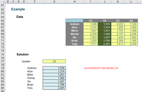
To show you how dynamic arrays can make the most of being able to create resultant vectors, consider the following example:

The formula

=XLOOKUP(G77,I65:L65,I66:L72)

 again resolves to a vector – but this time is allowed to spill as a dynamic array. Obviously, this will only work in Office 365, but it’s an especially useful tool that might just make you think it’s time to drop that perpetual licence.

Once you start playing with the dynamic range side, you can start to get imaginative. For example:

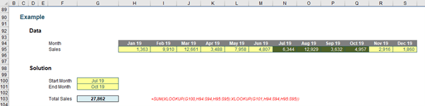
In this illustration, I want to calculate the sales between two periods:

This might seem like a simple drop-down list using data validation (ALT + D + L), but XLOOKUP has been used in determining the list to be used for the end months.

Let me explain. I have hidden the range of relevant dates in cell H101 spilled across

01

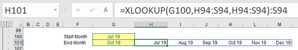
XLOOKUP can return a reference, so the formula

=XLOOKUP(G100,H94:S94,H94:s94):S94

 evaluates to the row vector N94:S94 (since the start month is July). This spilled dynamic array formula is then referenced in the data validation:

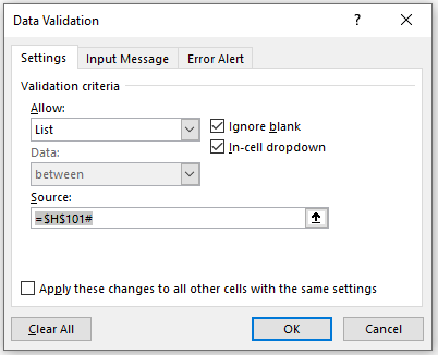
(You may recall $H$101# means the spilled range starting in cell H101.)  It should be noted that the formula =XLOOKUP(G100,H94:S94,H94:s94):S94 may not be used directly in the ‘Data Validation’ dialog, but this is a neat trick to ensure you cannot select an end month before the start month (assuming you are a rational human being that selects the start before the end!).

The formula to sum the sales then is

=SUM(XLOOKUP(G100,H94:S94,H95:S95):XLOOKUP(G101,H94:S94,H95:S95))

Again, this uses the fact XLOOKUP can return a reference, so this formula equates to 

=SUM(N95:Q95)

Easy!  Now I am combining two XLOOKUP formulae with a colon (:) to form a range.  This joins other illustrious functions used this way such as CHOOSE, IF, IFS, INDEX, INDIRECT, OFFSET, SINGLE (@), SWITCH and TEXT.  First nesting, now joining – what’s next?