Calculating car financing rates

You may be surprised to learn I am not a multi-millionaire (or even a single one). This fact seems lost on my beloved daughter. Money clearly grows on financing trees so I had to go cap in hand to get a loan for her car – and I wasn’t convinced the rate I was being quoted was correct. Therefore, I decided to recalculate it myself.

Two birds killed with one stone: dispute raised with financing company and article written for ICAEW!

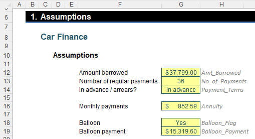
Let’s imagine I am seeking to finance a car over 36 months and the amount to be financed is $37,799 with monthly repayments in advance of $852.59 with a final (“balloon”) repayment of $15,319.60 at the end (hmm… sounds suspiciously like quoted numbers). Imagine you were told the rate implicit in the loan was 6.99% p.a. Is this correct?

Microsoft proposes you can use RATE to determine the implicit rate here.

As a piece of revision here, annuities often need to be calculated, ie, regular, periodic payments of identical amounts earning a similar rate of return.

Perhaps the easiest way to think of it is as follows:

• Let’s assume interest is set at 10% (and we will assume this is after tax)
• Something that is invested at $100 this year will increase by 10% next year, ie, be valued at $110
• Something that is invested at $100 this year will increase by 10% over the next two years, ie, be valued at $121
• Something that is invested at $100 this year will increase by 10% over the next three years, ie, be valued at $133.10. etc.

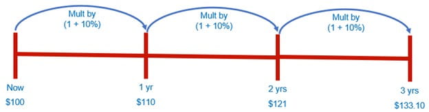
Note that all of these valuations are for a point of time not a period. This is a common mistake in modelling.

The RATE function returns the interest rate per period of such an annuity. RATE is calculated by iteration and can have zero [0] or more solutions. If the successive results of RATE do not converge to within 0.0000001 after 20 iterations, RATE returns the #NUM! error value.

The RATE function has the following syntax:

RATE(nper, pmt, pv, [fv], [type], [guess])

The RATE function has the following arguments:

• nper: this is required and represents the total number of payment periods in an annuity
• pmt: this is also required. This is the payment made each period; it cannot change over the life of the annuity. Typically, pmt contains principal and interest but no other fees or taxes. If pmt is omitted, you must include the pv argument
• pv: this argument is also required. This is the present value, or the lump-sum amount, that a series of future payments is worth right now. If pv is unspecified, it is assumed to be zero [0]
• fv: this argument is optional and represents the future value, or a cash balance, you want to attain after the last payment is made. If fv is omitted, it is assumed to be zero [0] (the future value of a loan, for example, is 0). If fv is omitted, you must include the pmt argument (which is a weird thing to say given it is required!)
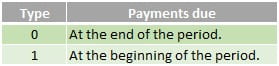
• type: this is also optional. The type should either be zero [0] or one [1] and indicates when payments are due. If type is omitted, it is assumed to be zero [0]

• guess: another optional argument. Your guess for what the rate will be. If you omit the guess, it is assumed to be 10%. If RATE does not converge, try different values for guess. RATE usually converges if guess is between zero [0] and one [1].

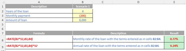
Make sure that you are consistent about the units you use for specifying guess and nper. If you make monthly payments on a four-year loan at 12% annual interest, use 12%/12 for guess and 4*12 for nper. If you make annual payments on the same loan, use 12% for guess and 4 for nper.

For all the arguments, cash you pay out, such as deposits to savings, is represented by negative numbers; cash you receive, such as dividend receipts, is represented by positive numbers. As an example:

Sometimes, the numbers aren’t quite what you expect for this function. That’s because Microsoft uses the following relationship to be consistent across its related financial functions:

Unfortunately, in this instance, this seems to be one of those times when the RATE function will let us down – so we will need to construct it from first principles. Time for the attached Excel workbook!

In this workbook, I have detailed the aforementioned assumptions and given the cells range names, viz.

Cell G14 (Payment_Terms) has a data validation dropdown list (ALT + D + L) with the options of “In advance” or "In arrears”; cell G18 (Balloon_Flag) has a similar feature but with the values “Yes” and “No”. If the Balloon_Flag is set to “No” then Balloon_Payment (cell G19) is formatted to be blank and ignored.

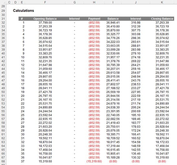
We can now create a Calculations Table:

To the eye, it probably won’t take you too long to follow the logic but allow me to explain the formulae in each column so that you may replicate and understand the calculations.

Column E (#) lists the period numbers. There are 36 regular payments, plus a final balloon payment, which means there are 37 periods in total. This can be summarised by the formula in cell E32:

=SEQUENCE(No_of_Payments + (Balloon_Flag = "Yes"))

The formula No_of_Payments + (Balloon_Flag = "Yes") calculates the number of periods, namely 36 plus one [1] more if there is a balloon payment at the end. The formula effectively resolves to SEQUENCE(37), which is a dynamic array formula which puts the numbers one [1] to 37 down a column.

If you are not working in Excel 365 or Excel on the web, you may not be able to use this so-called dynamic array formula. Alternative calculations such as

=IF(MAX($E$31:$E31) = No_of_Payments + (Balloon_Flag = "Yes"), "", MAX($E$31:$E31) + 1)

will have the same effect and may still be copied down to more rows. For simplicity, I will have this formula as my only dynamic array calculation in the table.

Column F (Opening Balance) calculates, er, the opening balance. For example, the formula in cell F32 is given by

=IF($E32="", "", IF($E32=1, Amt_Borrowed, K31))

The first IF expression, =IF($E32="", "", …), will be used throughout Calculation Table to check that the period number exists – if it is blank, no calculation should be computed. The remainder of the formula, IF($E32=1, Amt_Borrowed, K31), simply checks if it is the first period: if so, the Amt_Borrowed (here, $37.799) is entered, otherwise it is the closing balance of the previous period. You can note this can never cause an error because there is always a previous closing balance for periods 2 onwards.

The next column, column G (first column called “Interest”), calculates the interest if and only if the payment is made at the end of the period (ie,. Payment_Terms are “In arrears”). Thus, the formula in cell G32 is

=IF($E32="", "", IF(Payment_Terms = "In advance", 0, F32 * Monthly_Rate))

To be clear, the formula is actually checking whether Payment_Terms are “In advance” (and hence the amount will be zero [0]), otherwise it is taking the Opening Balance (cell F32) and multiplying it by the Monthly_Rate, which is the monthly interest rate implicit in the loan.

Erm, hang on a minute: Monthly_Rate? This hasn’t been defined yet. I am going to name cell G21 Monthly_Rate:

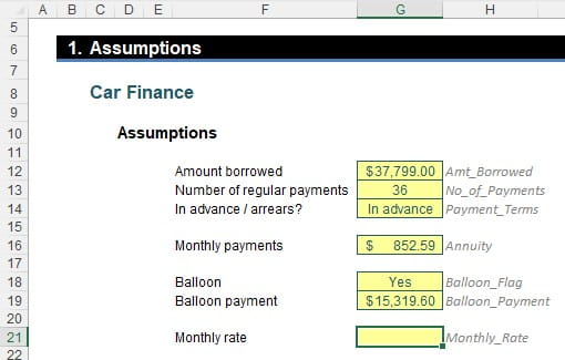
If you are wanting to get the same numbers as in my example, you might want to set Monthly_Rate to be the value

0.857956023745794%

or some similar rounded number on order to get the same values. Don’t worry, we will work this value out later!

Next, the Payment column (column H) calculates the regular payment (ie, the Annuity or the Balloon_Payment in the final period if necessary). Hence, the formula in cell H32 is

=IF($E32="", "", -IF($E32 = No_of_Payments + 1, Balloon_Payment, Annuity))

Assuming this is a calculating period, this formula checks to see if the period number (column E) is equal to one more than the number of annuity payments; if so, it enters the negative value of the Balloon_Payment, otherwise it records the negative value of the Annuity.

Some of you might wonder why we are not checking to see whether there is a balloon payment. There is no need: if Balloon_Payment is set to “No”, the period counter will end at 36, not 37, and the condition IF($E32 = No_of_Payments + 1, … cannot be fulfilled. Keep your formulae simple!

The next column, Balance (column I) is simple, with the formula in I32 equal to

=IF($E32="", "", SUM(F32:H32))

This calculation should be self-explanatory: it simply adds the Opening Balance, the first amount of Interest and the Payment made together.

Column J (second column called “Interest”), calculates the interest if and only if the payment is made at the beginning of the period (ie, Payment_Terms are “In advance”). Thus, the formula in cell J32 is

=IF($E32="", "", IF(Payment_Terms = "In advance", I32*Monthly_Rate, 0))

You can clearly see if the Payment_Terms are “In advance” the formula is taking the Balance just calculated (cell I32) and multiplying it by the Monthly_Rate, otherwise the value is zero [0].

The final column, column K (Closing Balance) is then simply the sum of the interim Balance and the second computation for Interest. Therefore, for cell K32, we have the formula

=IF($E32= "", "", I32 + J32)

This is simply copied down to the final period (or beyond if you want to flex the number of periods). If you have used the Monthly_Rate I suggested, you should have the following result:

You can manually change the Monthly_Rate to achieve a final balance of (approximately) zero [0] – or you can use Excel’s built-in functionality, ‘Goal Seek’.

To do this, I have added a formula for the Final Balance into cell K21:

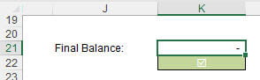
The formula is given by

=ROUND(OFFSET(K31, No_of_Payments + (Balloon_Flag = "Yes"), 0), Rounding_Accuracy)

If you look at the previous image, you will note that cell K31 is the header for the Closing Balance column. The OFFSET function moves the reference No_of_Payments + (Balloon_Flag = "Yes") rows down (ie, the total number of periods of the loan) which will be the final Closing Balance, which is then rounded to zero [0] decimal places. This is because the range name Rounding_Accuracy has a value of zero [0] in our attached Excel file.

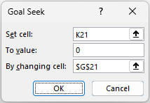
Therefore, to calculate the rate implicit in the loan, we need to find the value of Monthly_Rate which makes this value zero [0]. And that’s where Goal Seek comes in.

Goal Seek (ALT + A + W + G, or else go to the Data tab on the Ribbon, then in the Forecast group, select ‘What-If Analysis’ and then choose ‘Goal Seek…’) requires three inputs:

The ‘Set cell’ value is the Final Balance output here, ‘To value’ is the desired outcome (eg, zero [0]) and ‘By changing cell’ defines the variable input (here, the Monthly_Rate). This should give the value cited earlier. You can turn this into a macro should you wish (the Excel file does go this far).

Finally, we need to calculate the Annual_Rate (cell G22):

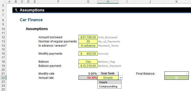
The formula here depends upon whether we select “Simple” or “Compounding” for the annualisation methodology. If you are going to pay off the car, then the payment must exceed the interest, so “Simple” should really be what you choose, but I include both options for completeness and my CDO disorder (it’s like OCD, Obsessive Compulsive Disorder, but I need the letters in alphabetical order!). Therefore, the formula in cell G22 is given by

=IF(H22="Compounding",

(1 + Monthly_Rate) ^ Months_in_Year - 1,

Monthly_Rate * Months_in_Year)

This either uses the standard compounding formula or else multiplies the Monthly_Rate by 12 (Months_in_Year). Clearly, our rate is not 6.99%; it is actually 10.30%. Hmmm…

Word to the Wise

Hopefully, a key point raised in this article is to lay out workings and computations as simply as possible. Sometimes, Excel functions (such as RATE) will fail due to their underlying assumptions and hence not provide you with the desired result. You can always fall back on first principles which is what has happened in this instance.

Calculations with five [5] or more periods are not always solvable using mathematical formulae. There are times when good old ‘Goal Seek’ may need to be utilised instead. This may lead to a “black box” solution so always check the value Excel offers you works. It may be verified here, as we can clearly see the Final Balance is zero [0].

Finally, do note that the quoted interest rate on a loan doesn't always reflect the true cost of financing because it doesn't necessarily account for all fees and charges associated with the loan. Lenders will always try to make things look cheaper in a highly competitive marketplace: always reconstruct total fees and costs to obtain a more accurate picture regarding the total cost of borrowing. But then you know that!