Listing Duplicates

It’s easy enough to remove duplicates in Excel (Date -> Remove Duplicates is one such way), but what happens when you wish to create a dynamic list of duplicates that can distinguish between items with leading zeroes? That’s a lot trickier. This month, I plan to generate a list of duplicates from the original list containing a mix of “real” numbers, numbers with leading zeroes and numbers in text strings.  

You can finally get your telephone and credit card lists sorted!

I make no apologies for using Excel 365 features today. Dynamic arrays have just celebrated their seventh birthday in Excel (today, in fact, as I write!). If you still don’t have dynamic arrays, I really do think it’s high time you upgrade. There is a good chance the version of Excel you are working on will no longer be supported by Microsoft in less than a month’s time.  

Numbers with leading zeroes may sometimes cause problems. In order to find duplicates from a list, you might think of using FILTER with COUNTIF. However, COUNTIF cannot distinguish between numbers with and without leading zeroes, or “numerical” numbers and numbers stored as text or else in text format.

As you can see below, the number of occurrences of each number is calculated incorrectly by COUNTIF:

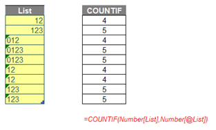
The green comments in the left-hand top corner of the yellow (assumption) cells have been retained deliberately as they highlight these entries are numbers stored as text. Therefore, this challenge was trickier than it may have first appeared. You can download the number list in our attached Excel file.

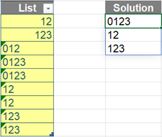
I am going to write a formula in one cell using dynamic arrays that will spill down a column to generate a list of duplicates (i.e. all numbers that show up more than once) from the number list in the file above. The result had to be similar to the list on the right (below):

As already stated, you can find my Excel file here which demonstrates my suggested solution.

When finding duplicates, you may think of some of the following common ways:

• COUNTIF / COUNTIFS
• SUMPRODUCT
• EXACT
• conditional Formatting to highlight duplicates
• etc.

However, after trying all the options above, you will realise that they do not seem to meet the requirements of the question – at least easily.

For example, if we use dynamic arrays with COUNTIF, the result may be wrong. As numbers 12 and 123, and string “012” only show up once in the list, they should not be considered as duplicates.

Before explaining my solution, allow me to clarify how I came up with it first.

Brainstorming

The aim here is to count the number of occurrences of each number in the list to check whether those numbers were considered as duplicates or not.

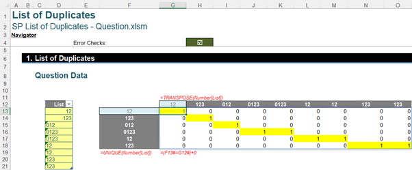
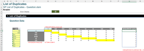
Firstly, I’m thinking of using a matrix with:

• x axis being the Number list (i.e. G12#) with the help of TRANSPOSE
• y axis being its unique list (i.e. F13#) with the help of UNIQUE
• counting only numbers from the unique list is enough.

The values in the matrix will be 1 (TRUE) or 0 (FALSE) depending on whether numbers on the y axis show up on the x axis (i.e. the number list) or not.

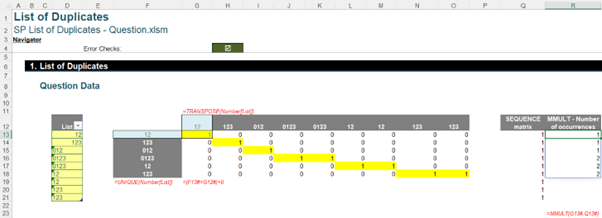
Secondly, I need to sum up each row of the matrix to get the frequency each number show up. As you may know, I cannot use SUM with dynamic arrays to calculate each row’s result as it will aggregate the result of all rows. Hence, I will apply a trick with the MMULT function (see below) to multiply the matrix above by a matrix containing only number ones [1’s]

The second matrix is created by SEQUENCE which I have written about previously. The number of rows of this matrix needs to be the same as the number of columns of the first matrix above. The formula is as follows:

=SEQUENCE(COLUMNS(G13#),,,0)

The syntax of the MMULT function is as below.  It will return the matrix product of two specified arrays or matrices:

=MMULT(array1, array2)

Hence, I will get a result matrix on column R below, which is a list of the number of occurrences:

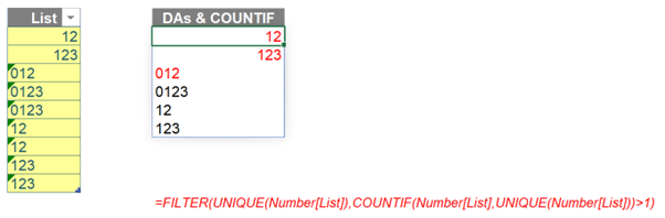
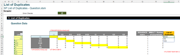
Finally, I just need to use the FILTER function to remove all the numbers which only occur once:

=FILTER(F13#,R13#>1)

Putting it Together

Sometimes it’s worth putting a formula into one cell – condense it, so to speak – as helper cells can be confusing for end solutions. Therefore, my formula is a combination of all steps above within a LET formula as follows:

=LET(List,Number[List], Matrix,(UNIQUE(List)=TRANSPOSE(List))+0,
FILTER(UNIQUE(List),MMULT(Matrix,SEQUENCE(ROWS(List),,,0))>1))

There are two variables, namely List and Matrix. List is the original number list in the question, whereas matrix is the first matrix to calculate the number of occurrences. Then, the final part of the formula is the calculation to get the list of duplicates, viz.

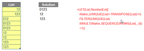
Although it is a long and complex formula, you can apply it to your own list by only replacing the value (i.e. Number[List]) of the variable List.

Word to the Wise

The eagle-eyed will note the curious addition of zero (“+0”) in the final formula. This forces values and also ensures recalculation. Just another Excel trick to add to the kitbag!