
Sometimes, when you work with pivoted data that has a structure similar to what would be generated if you had created a PivotTable, it is difficult to look up a value based upon multiple column and row criteria. To make it simpler, we usually unpivot the data. Most of the time, you might choose to use ‘Unpivot columns’ function in Power Query – but sometimes, it’s better to go with a dynamic (ie, updates automatically) formula.
Power Query alternative
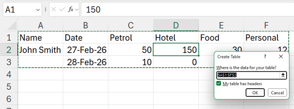
Let’s imagine PQ_Example_CSV has come in, and it is an expense csv which is not in the usual format because our claimant (John Smith) has configured his data ready to create a graph of where his expenses go. Convenient for him, but not so great for possible analysis:
| Name | Date | Petrol | Hotel | Food | Personal |
| John Smith | 27 Feb 26 | 50 | 150 | 30 | 12 |
| 28 Feb 26 | 10 | 0 | 25 | 0 |
Luckily, Power Query has a button for this – in order to get this into our required column format we will need to unpivot the data. The first step is to open this expense CSV and click somewhere in the table in the Excel workbook.
Choose to create a new Power Query, in this case From Table. A pop-up will appear to confirm the boundaries of the table – adjust this range if required. There is also a check box to indicate whether the table has headers:
Clicking ‘OK’ allows the data to be edited in the ‘Power Query Editor’ window as shown below:
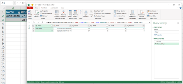
The first step for this example is to remove any unnecessary data – in this case John has added a personal expense column which is not required in the model. We could highlight the column and either use the ‘Remove Column’ option on the Home tab, or right-click and choose Remove.
The name can then be filled down by highlighting the Name column and using the ‘Fill Down’ option on the ‘Transform’ tab.
Finally, the unpivot process - select any columns to be ‘unpivoted’ (holding down SHIFT) – in this example this is everything except Name and Date. In the ‘Any Columns’ group on the ‘Transform’ tab there is an option to ‘Unpivot Columns’ – there are several options, but I will select the Name and Date fields and choose ‘Unpivot other columns’ in case there are other columns next time:
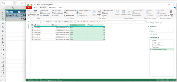
One click and everything is unpivoted as required! The problem here is should the data be modified, you will have to refresh the query – and many end users forget to do this.
Formulaic approach
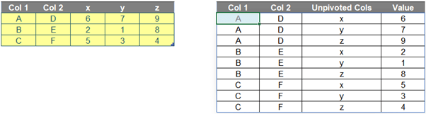
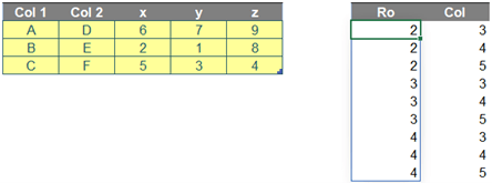
This can be done automatically by simply writing a formula in one cell using dynamic arrays. This is probably preferable. This approach would spill a range of cells to unpivot only the last three [3] columns (ie, x, y and z) of the array in the file above. The result should look like the array generated on the right (below):
To construct our calculation, we will need to consider the following:
- The table of data, turned into an Excel Table (CTRL + T), called Table
- number of columns that will not be unpivoted, which is two [2] (ie, Col 1 and Col 2). We will name it as ColstoKeep.
Therefore, the number of columns to unpivot is three [3], which is calculated as below. We name this number as UCols.
=COLUMNS(Data[#All]) - ColstoKeep
Secondly, we need to consider some features (eg, numbers of rows and columns) of the output array. After we unpivot the table, they should be calculated as below:
- Number of rows: 9
=(ROWS(Data[#All]) - 1) * UCols
- Number of columns: 4. The output table will include the first two [2] columns of initial table and two [2] additional columns for the old Row Headers (ie, x, y and z) and Values (ie, numbers in Data table in this case).
=ColstoKeep + 2
Thirdly, to create a Dynamic Range for the output, we need the help of INDEX and SEQUENCE.
The row and column index numbers of output need to be created by SEQUENCE as follows. We will call them RowID and ColID.
- RowID:
=SEQUENCE((ROWS(Data[#All]) - 1) * UCols)
- ColID:
=SEQUENCE(1, ColstoKeep + 2)

Additionally, we need to identify row and column positions of the Values in Data. We will call them Ro and Col.
For example, number ‘7’ is located on row 2 and column 4 of Data.
- Ro:
=ROUNDUP(RowID/UCols,0)+1
- Col:
=MOD(RowID-1,UCols)+1+ColstoKeep
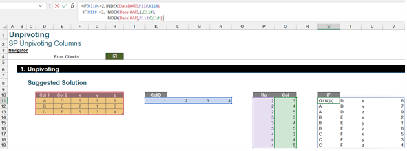
Finally, the trick of this challenge is to use ColID with an IF statement (below) as a connector for three different INDEX functions, ie,
“If ColID is less than or equal to ColstoKeep, then get the first two [2] columns of Data, else if ColID is equal to ColstoKeep + 1, then get the Row Header of unpivoted columns of Data, else get the Values of Data.”
The result is as follows:
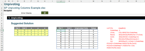
You may wonder why the challenge only allows a formula cell when there are several working steps above. Our solution is a combination of all described steps above within a LET formula as follows:
LET(Tbl, Data[#All],
ColstoKeep, 2,
UCols, COLUMNS(Tbl)-ColstoKeep,
RowID, SEQUENCE((ROWS(Tbl)-1)*UCols),
ColID, SEQUENCE(1,ColstoKeep+2),
Ro, ROUNDUP(RowID/UCols,0)+1,
Col, MOD(RowID-1,UCols)+1+ColstoKeep,
IF(ColID<=ColstoKeep,INDEX(Tbl,Ro,ColID),
IF(ColID=ColstoKeep+1,INDEX(Tbl,1,Col), INDEX(Tbl,Ro,Col))))
There are seven [7] variables:
- Tbl is an input table to unpivot
- ColstoKeep is the number of first columns you do not want to unpivot
- UCols is the number of unpivoted columns
- RowID and ColID are row and column indices of the output table
- Ro and Col are initial row and column positions of Values in the input table.
Then, the final part of the formula is the calculation to unpivot the last three [3] columns, viz.
Although it is a long and complex formula, you can apply it to your input table by only replacing the values of Tbl and ColstoKeep. Simple!
Archive and Knowledge Base
This archive of Excel Community content from the ION platform will allow you to read the content of the articles but the functionality on the pages is limited. The ION search box, tags and navigation buttons on the archived pages will not work. Pages will load more slowly than a live website. You may be able to follow links to other articles but if this does not work, please return to the archive search. You can also search our Knowledge Base for access to all articles, new and archived, organised by topic.
