Conditional formatting and spreadsheet review – one rule to find them all

How to Review a Spreadsheet takes a very practical look at how to identify possible issues with a spreadsheet and thereby reduce the likelihood of errors occurring and improve overall efficiency. The webinar that launched the project not only presented an overview of the importance, purpose and structure of the publication, but the lead author, John Tennent, also covered a range of easy and practical ways to uncover problem areas and deficiencies in any spreadsheet.

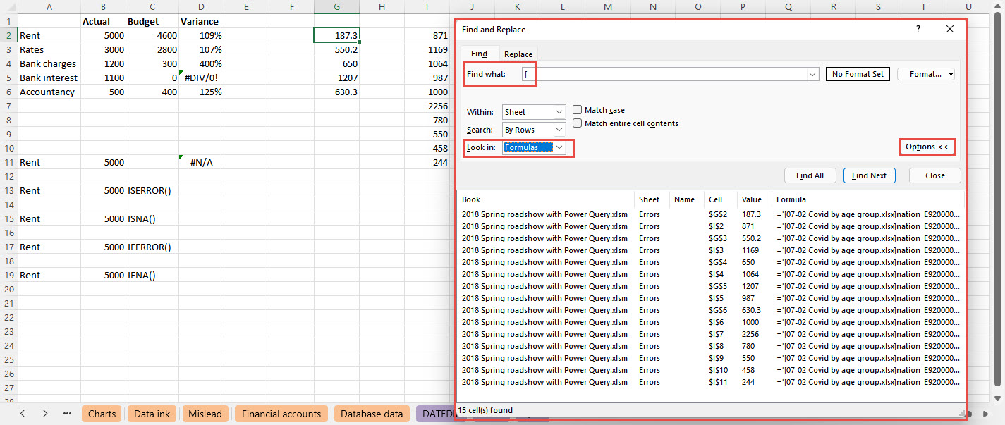
One such method featured the use of the Excel Find command to identify all cells linked to an external workbook by finding cells that contained an opening square bracket. Using Find All, this could display a list of all such cells to work through. Note that in this screen shot we have clicked on the Options button which allows us to define where we are searching and to ensure that we are looking in Formulas:

In a related question, one of the participants asked about possible ways to detect the use of the IFERROR() function which can potentially mask important errors. Of course, in the same way that Find can be used to seek out the square bracket in a formula, it could also be used to find cells that use a particular function. At this stage it's worth pointing out that IFERROR() is just one of several functions that can be used to mask errors or other issues. Most generally, IF(), IFS() and SWITCH() can all be used to replace any value with an alternative value but there is also a range of error checking functions. Before Microsoft added the likes of IFERROR() and IFNA(), the equivalent ISERROR() and ISNA() had to be combined with IF() to check for errors. Both ISNA() and IFNA() are more specific than ISERROR() and IFERROR(). Where the latter two functions would mask any error in a function that included one of the lookup functions, the 'NA' functions would still report errors apart from #N/A, as errors.

As the review publication mentions, some very useful software diagnostic tools are available to highlight particular cell contents and states and the following exploration of conditional formatting capabilities is not intended to replace other, more capable, tools but instead to demonstrate how conditional formatting can be used for more than just highlighting ranges of values in a workbook.

We are going to create a conditional format that uses a formula, and that formula will use the FORMULATEXT() function to examine the formula in each cell, rather than the result. We will also be using the SEARCH() function to look for particular formula contents. Note that Excel has two very similar functions for finding a text string within another text string: SEARCH() and FIND(). SEARCH() is not case-sensitive whereas FIND() is.

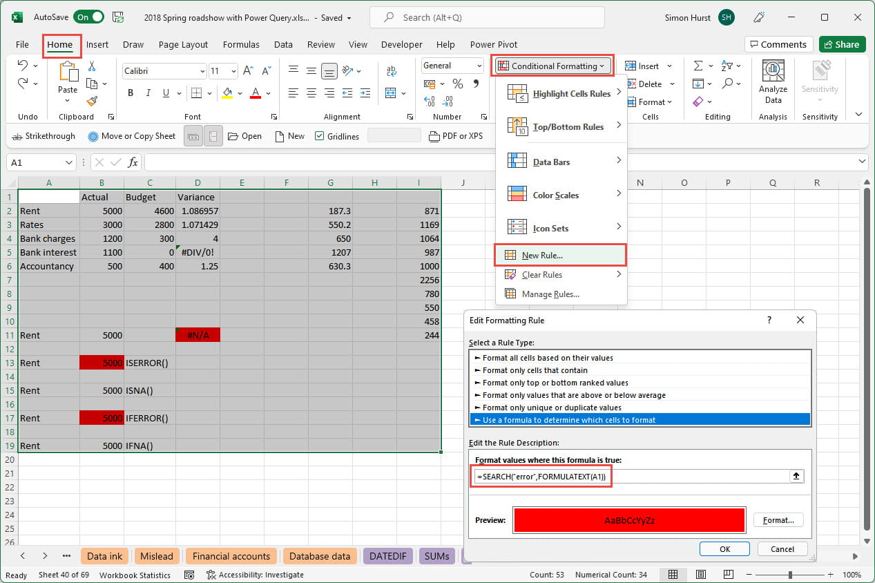
Here, we have clicked on New Rule… from the Home Ribbon tab, Styles group, Conditional Formatting dropdown. We have chosen to 'Use a formula to determine which cells to format' and, with the range of cells that we want to check selected, entered the following formula, where A1 is a relative reference to the top left-hand cell of our selection:

=SEARCH("error",FORMULATEXT(A1))
We have set our Format to a Red Fill and we can see that three cells have the format applied to indicate the presence of 'error' somewhere in the formula:

The SEARCH() and FIND() functions return the starting position of the first occurrence of our search term within our formula. If the term is not found, a #VALUE! is returned. In a conditional format formula positive and negative numbers (apart from 0) equate to TRUE, whereas an error value is not TRUE (or FALSE for that matter). Accordingly, we don't need to complicate our Conditional Formatting formula by using IF() to see whether our formula returns a number or an error, as only something that evaluates as TRUE will trigger the format.

So far, we have seen how to use conditional formatting to highlight cells based on a part of the content of the formulae they contain. Next time we will examine various ways of coping with multiple conditions as well as the implementation of a kill switch.