Conditional formatting and spreadsheet review – part two

In part one we looked at combining the use of the FORMULATEXT() function with conditional formatting to highlight cells where the formula contained some sort of content that we wanted to highlight as part of a spreadsheet review, such as links to external workbooks or the use of particular functions. This time we are going to consider taking the idea further to incorporate searching for multiple items and being able to turn our review conditional formatting on and off.

We can use the logical functions AND() and OR() to apply the same format for multiple checks but, if we want to use OR(), we can't rely on the TRUE/FALSE shortcut described in part one. One error value in our set of tests will result in an overall error value result, so OR() will work like AND() in that a single error value will mean that the overall result is an error and therefore not TRUE. Instead, we can use the ISNUMBER() function to convert any error value to 0 and non-errors to 1:

=OR(ISNUMBER(SEARCH("error",FORMULATEXT(A1))),ISNUMBER(SEARCH("if",FORMULATEXT(A1))))

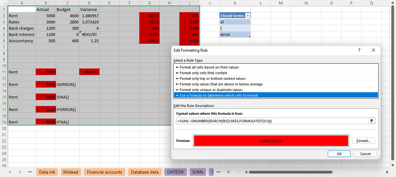
In the era of dynamic arrays, we can make things much simpler to set up and much easier to adapt. We can enter our 'OR' terms in a block of cells and refer to that block of cells:

=SUM(--ISNUMBER(SEARCH($K$3:$K$5,FORMULATEXT(A1))))

Here, we use ISNUMBER() to convert our error values to FALSE, we then use the double minus to convert our TRUEs and FALSEs to 1s and 0s. Because dynamic array behaviour will calculate a value for each of our search terms, we use SUM() to add these values up. For Excel versions prior to the introduction of Dynamic Arrays the SUMPRODUCT() function could be used to force the array behaviour. If one or more of our searches returns a starting position number, rather than the #VALUE! error, then the overall sum will be a number and our conditional format criterion will return TRUE, so acting as an OR condition, and applying the chosen format:

It's worth pointing out that conditional formatting suffers from the same inconsistent behaviour as data validation when it comes to expanding Tables. If our Table of check terms is on the same sheet as our conditional format, adding rows with additional terms to our Table will automatically change the SEARCH() range in our conditional format formula. However, if the format and Table are on different sheets the range will not update in the same way. For this reason, it is better to apply an Excel Range Name to the Table column and use this in the conditional format formula. The formula should then adapt wherever in our workbook it is used.

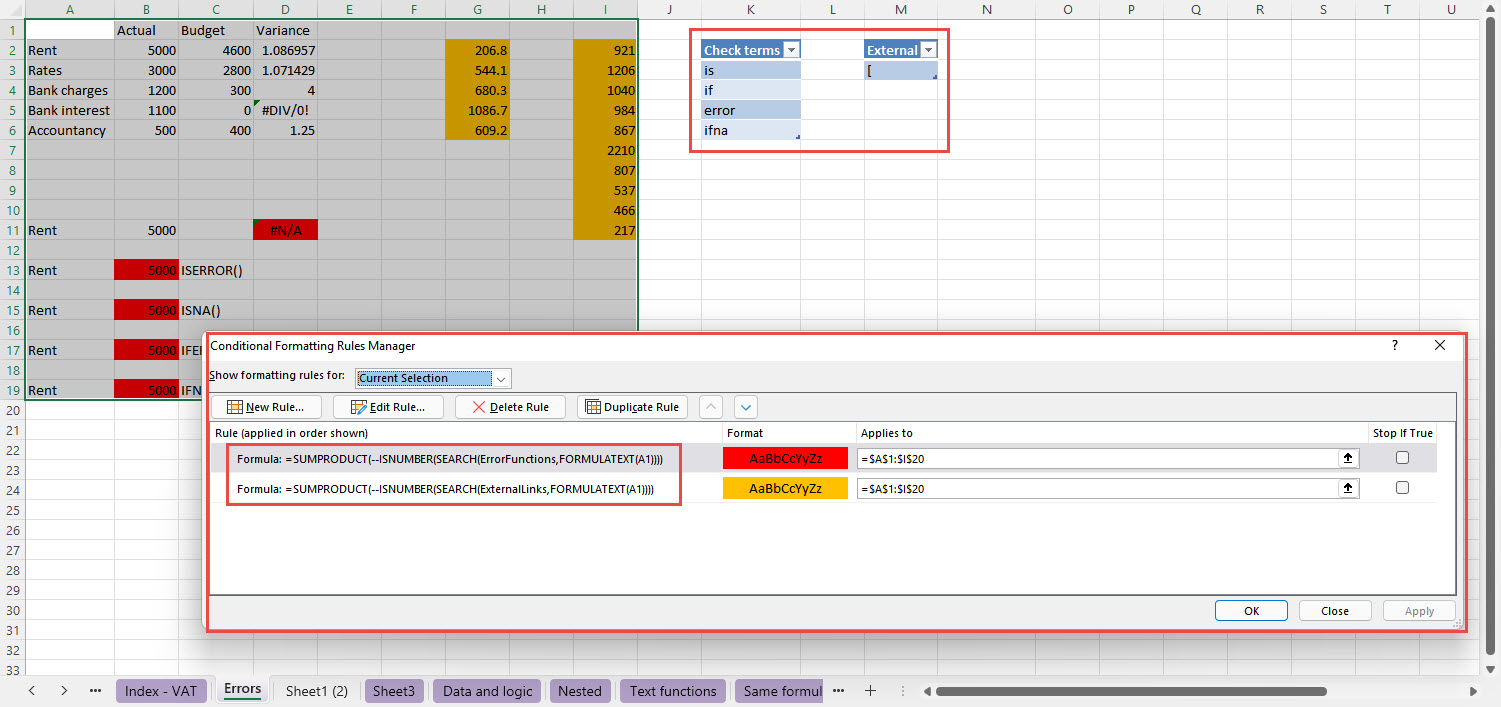
So far, we have set up a single conditional format that is applied dependent on multiple search terms, but we can also set up multiple conditional formats that apply the same, or different formats, based on different criteria.

Here, we have added a second Table, this time to find links to external workbooks using the open square bracket formula as detailed in the launch webinar for the new Spreadsheet Review publication. We have applied Range Names to the columns of each Table and then edited the existing conditional format to use the Range Name rather than cell range. We have then gone to Conditional Formatting, Manage Rules…, Duplicate Rule to create a copy of our existing rule. We can then select our new rule and choose Edit Rule… in order to change the Range Name to refer to the Range Name for our second Table and to choose a different fill colour:

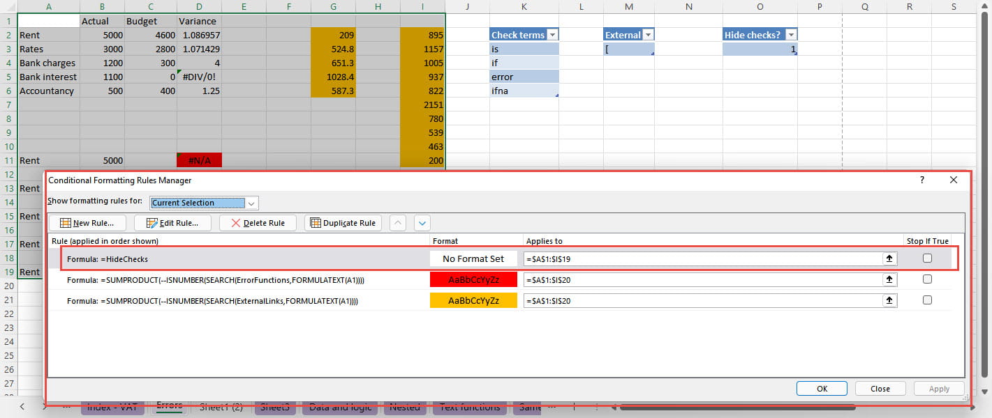
Finally, we will look at being able to turn these review conditional formats off easily so that we can continue to view and print the spreadsheet without them. We will do this by setting up another conditional format which will include no format settings, but which is designed to hide our review conditional formats. This new conditional format rule will again be based on the contents of a named cell. In this case we will use a single cell that contains TRUE or FALSE or a value that equates to TRUE or FALSE and allocate the Range Name 'HideChecks'. We will use the New Rule… option to add a rule that uses a very simple formula:

=HideChecks

If we just add this new rule to our list of rules, it will make no difference whether our HideChecks cell contains a TRUE or FALSE value, because all of our rules will still be applied:

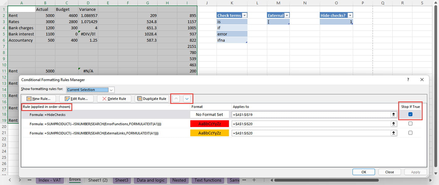
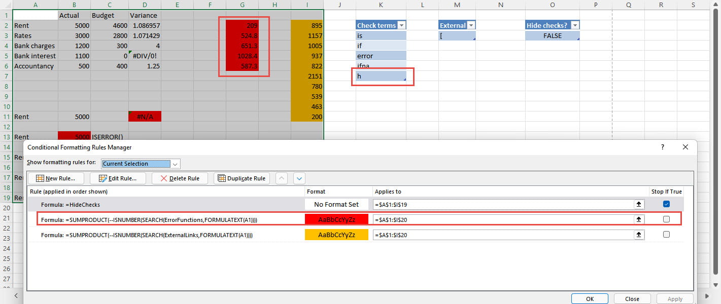
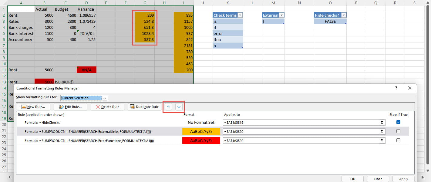
The key is the Stop If True option for each rule. If we turn on Stop If True for our new rule with No Format Set, then, when the criterion evaluates as TRUE, the rule will be applied, and further rules will not be used:

Note that the order of rules is crucial here. As the prompt in the first column header indicates, the rules are 'applied in order shown' so, for our set of rules to work as intended, our Checks rule needs to be at the top of our list of rules. Up and Down buttons allow us to move the selected rule. It is easy to misunderstand how the order of rule works. This is relevant where a particular format property is set by more than one rule. Obviously, in this situation, both rules can't be applied. You might expect that 'applied in order shown' means that Excel will work through the TRUE rules in order, with the rule lower down in the list thereby overwriting any earlier rules. In fact, the opposite applies. The rule higher in the list takes priority. We can see this in our example. If we change our search terms so that both of our review formats apply to certain cells, we will see that it is the format closer to the top of our list that is applied.

Here, we have added the search term 'h' to our Table of Check terms. The formulae in column G include references to column H in an external workbook so both our red and yellow fill formats apply. As we can see, it is the format closer to the top of our list that is applied: