
I was asked recently how to combine two different Sparkline charts in a single cell. This was one of those occasions when, although I came up with an answer that seemed to work, I couldn't help wondering whether there was an easier and better way.
If you know of one, please let us know at excel@icaew.com. The request was complicated by the need to create a column of Sparklines rather than an individual chart. If you haven't experimented with Sparklines, then one of the articles in John Tennent's Exploring Charts series provides a good introduction:
Simple methods such as trying to add two different Sparkline types to the same location failed: the second type of Sparkline just overwriting the first. Often, the solution to any requirement to overlay one part of a spreadsheet on another is the use of the Excel Camera and Linked Pictures. Once again, this feature has been covered in the past, most recently here:
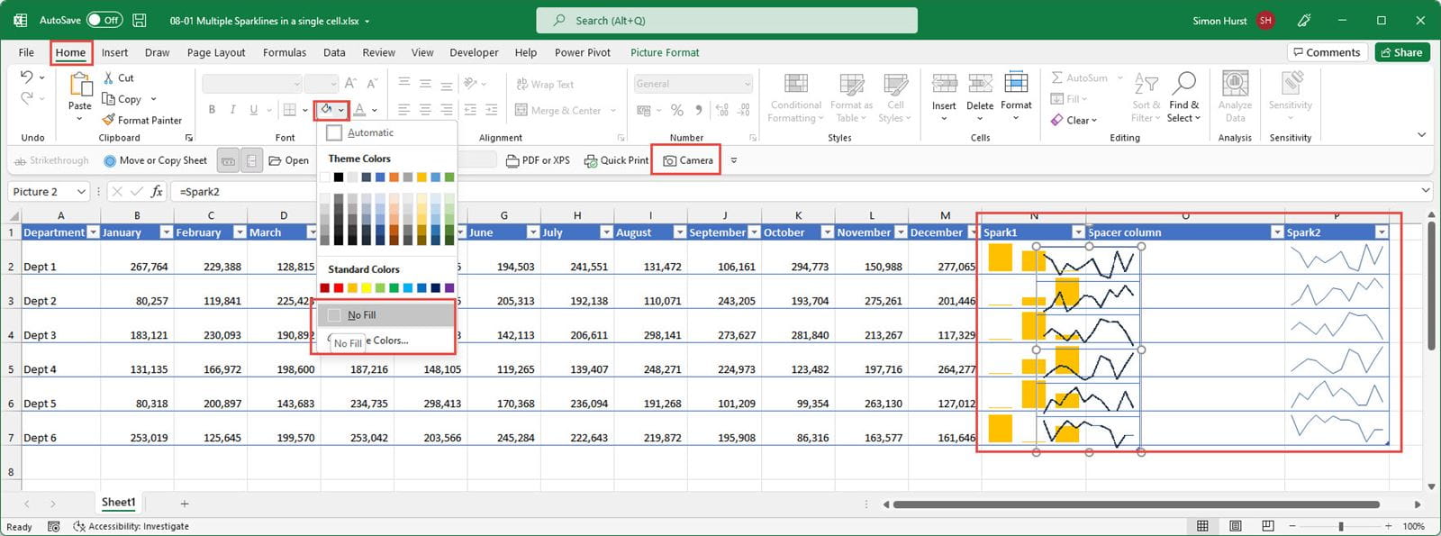
A Linked Picture is a graphic object that displays the contents of a cell or range of cells elsewhere in a workbook. Linked Pictures are dynamic, so that when the source content changes, the Linked Picture also changes immediately. To overlay a picture of a range of cells over other cells, the Fill colour of the Linked Picture needs to be set to No Fill. In this example, we have used an Excel Table with two columns containing different types of Sparkline. Just to demonstrate compactly how this works, our Column Sparkline displays the first three months results and our Line Sparkline the results for the whole year. In practical use, if you had 12 columns of actual results and 12 columns of budget results, you could use the technique to display the comparison of actual results against budget for example.
We want to create a Linked Picture of the Line Sparkline in cells P2:P7 of our Table. We can do this by adding the Camera command to our Quick Access Toolbar, selecting the cells, and then clicking on the Camera command. We can then Paste the resulting Linked Picture wherever we want it. Using the Home Ribbon tab, Font group, Fill Color dropdown we can set the fill to No Fill to make the background of the picture transparent:
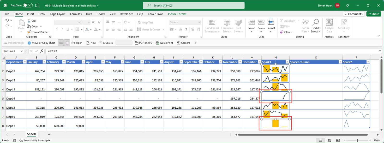
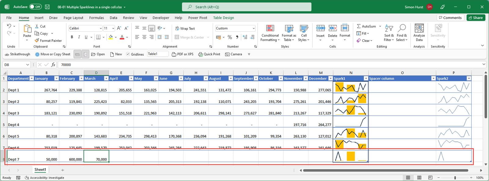
In order to allow for new rows, we need to change the data source for the Linked Picture from a fixed cell reference to a dynamic reference. We can create the dynamic reference using a Range Name for our Table column. Having undone our addition of the new Table row in order to return our Table to just 6 rows of data, we have created the Range Name "Spark2" to refer to cells P2:P7. The range referred to by the Range Name will change as rows are added to our Table.
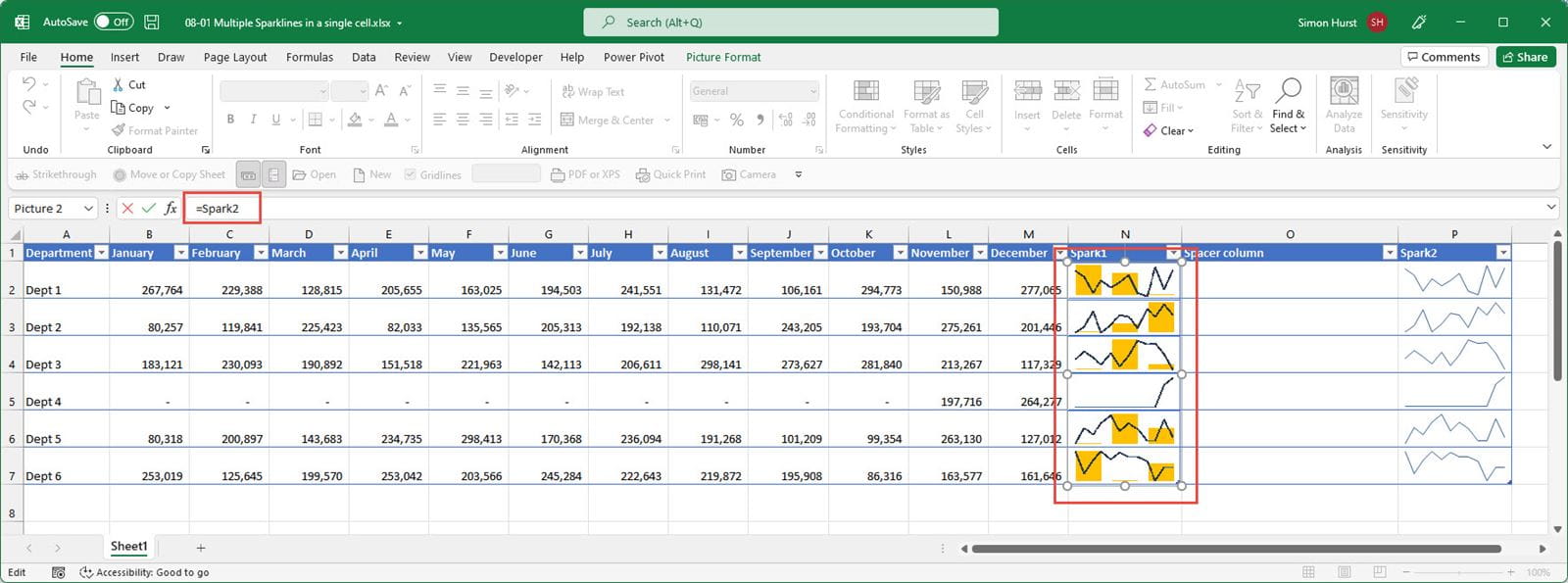
With our Linked Picture selected, the data source will be shown in the Formula Bar and we can replace our cell reference with the reference to the Range Name:
Join the Excel Community
Do you use Excel in your organisation? Are you using it to its maximum potential? Develop your skills and minimise spreadsheet risk with our Excel resources. Membership is open to everyone - non ICAEW members are also welcome to join.

Archive and Knowledge Base
This archive of Excel Community content from the ION platform will allow you to read the content of the articles but the functionality on the pages is limited. The ION search box, tags and navigation buttons on the archived pages will not work. Pages will load more slowly than a live website. You may be able to follow links to other articles but if this does not work, please return to the archive search. You can also search our Knowledge Base for access to all articles, new and archived, organised by topic.
