
The conditional aggregate functions such as SUMIFS() have long been some of the most useful functions for working with financial data, but they have their shortcomings and there might now be a more flexible and capable alternative.
In fact, this relates to a whole family of Excel functions including COUNTIFS(), AVERAGEIFS(), MAXIFS, MINIFS() and the predecessor functions SUMIF() and COUNTIF(). What all these functions have in column is the ability to calculate an aggregate value for a range of cells that is filtered by one or more conditions applied to the same range, or to a separate range with the same dimensions. The original SUMIF() and COUNTIF() functions allowed the use of a single criterion. SUMIFS(), COUNTIFS() and the other …IFS() extended this to allow the use of up to 127 pairs of separate criteria ranges and criteria values. This extension in the number of available criteria was significant, it meant that the functions could cope with more complex calculations such as extracting the total of values between two dates. The first criteria pair could compare a data column against the first value in the required date range, with the second pair comparing the same column against the last value in the range:
=SUMIFS(Invoices[Quantity],Invoices[OrderDate],">="&$A$2,Invoices[OrderDate],"<="&$B$2)
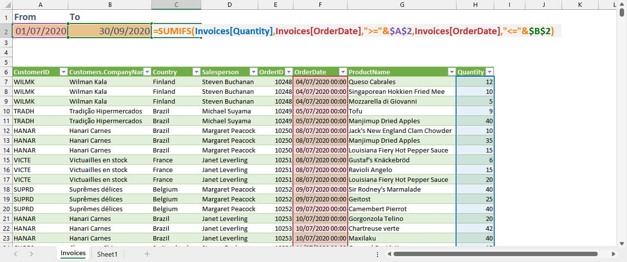
In this formula, we are working with a set of order transactions held in an Excel Table named ‘Invoices’. We need to calculate the quantity ordered between two dates using the OrderDate column. The first argument of our function is the range that we want to add up: Invoices[Quantity]. The next two arguments contain the first pair of criteria range and criteria value: the first criteria range is the column: Invoices[Quantity] and the first criteria value is:
">="&$A$2
We have entered the date in cell A2 and used the comparison operator >= to include all dates on or after the date entered. Note that we need to enter our comparison operator as a text string, surrounded by double quotes, and then use the & operator to concatenate this with the cell reference.
Our second criteria pair ensures that the total only includes dates on or before our To date:
"<="&$B$2
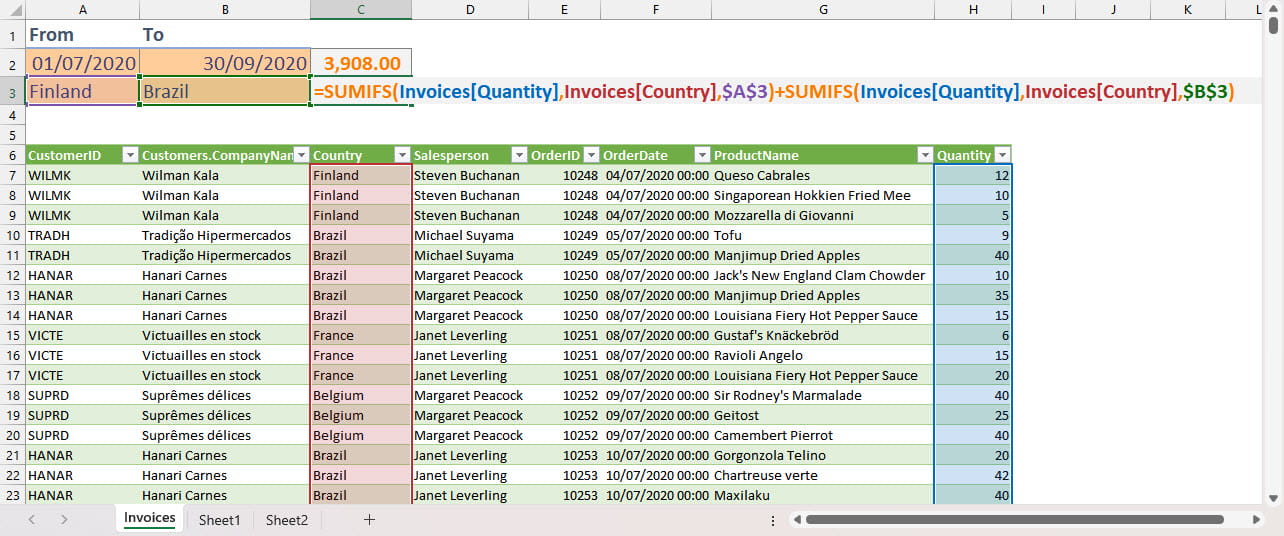
Although the ability to include multiple criteria significantly extends the usefulness of SUMIFS() and the related functions, there are still limitations. As we have seen, when referring to cells as part of a criterion that uses a comparison operator, the syntax is not obvious. Perhaps more importantly, the criteria operate only as an ‘AND’ filter and not ‘OR’. There are a few ways to use SUMIFS() to total values based on matching one criterion or another criterion, rather than having to match both, but the simplest is probably just to add two SUMIFS() formulae together:
=SUMIFS(Invoices[Quantity],Invoices[Country],$A$3)+SUMIFS(Invoices[Quantity],Invoices[Country],$B$3)
Another limitation is the inability to include other functions to change the values in the criteria ranges. For example, if, in our example, we wanted to total all the orders that had an OrderID value that started with 10 we would need to extract the first two characters of each of the values in the column using the LEFT() function. Attempting to embed the LEFT() function as part of any of the criteria ranges in a SUMIFS() formula will generate an error. We chose the OrderID column for this example because it contains numbers rather than text. If we wanted to use SUMIFS() to match the first part of the values in a text column, then we could just use the * wildcard:
=SUMIFS(Invoices[Quantity],Invoices[Country],$A$3&"*")
We could also overcome this problem and other similar problems by adding columns to our data that performed whatever manipulation we needed and then use those columns for our SUMIFS() criteria ranges.
In the new era of Dynamic Array equipped Excel, we have a different way of dealing with the need to calculate conditional aggregates: we can use the FILTER() function in combination with whichever aggregate function we want to use. Here are the previous SUMIFS() formula examples with their SUM(), FILTER() equivalents:
=SUMIFS(Invoices[Quantity],Invoices[OrderDate],">="&$A$2,Invoices[OrderDate],"<="&$B$2)
=SUM(FILTER(Invoices[Quantity],(Invoices[OrderDate]>=$A$2)*(Invoices[OrderDate]<=$B$2),0))
The FILTER() function takes up to 3 arguments. The first is the range to be returned, the second is an expression that evaluates to TRUE or FALSE or equivalent, and the third is the value to return if no values match the criteria expression. This third value is important. If SUMIFS() finds no matches it will just return 0 whereas FILTER() will return a #CALC! error if the third argument is not present. Having filtered the values in our first range, the SUM() function adds them up. Omitting the SUM() would return a list of each of the matching values in separate cells if there was enough room.
The criterion or ‘include’ argument can be a simple expression that evaluates as TRUE or FALSE, such as:
Invoices[OrderDate]>=$A$2
Note that, unlike in a SUMIFS() formula, there is no need to use the double-quotes and & operator.
Also unlike SUMIFS(), we can enter more complex expressions and use Boolean logic to combine AND and OR comparisons. Multiplying two conditions together is equivalent to AND (1*0=0), whereas adding two conditions together is equivalent to OR (1+0=1). It is even possible to combine multiple AND conditions with multiple OR conditions.
In our first example, both date conditions need to be satisfied so we multiply them together, being careful to enclose each separate statement in brackets:
(Invoices[OrderDate]>=$A$2)*(Invoices[OrderDate]<=$B$2)
For our OR example we add our two conditions:
=SUMIFS(Invoices[Quantity],Invoices[Country],$A$3)+SUMIFS(Invoices[Quantity],Invoices[Country],$B$3)
=SUM(FILTER(Invoices[Quantity],(Invoices[Country]=$A$3)+(Invoices[Country]=$B$3),0))
Finally, we’ll look at the way SUM() and FILTER() can overcome our issue with selecting the first two characters of the OrderID column values:
=SUM(FILTER(Invoices[Quantity],LEFT(Invoices[OrderID],2)=$A$3,0))
As you can see, FILTER() allows us to manipulate the contents of a criteria column using another Excel function. In this example we have assumed that we have entered our comparison value in A3 as text. Had we entered it as a number, we would have had to include the VALUE() function as well:
=SUM(FILTER(Invoices[Quantity],VALUE(LEFT(Invoices[OrderID],2))=$A$3,0))
For our other aggregates, we can just replace SUM() with the appropriate functions such as COUNT(), AVERAGE(), MAX() or MIN(), or indeed some of the more exotic statistical functions.
For simple conditions using SUMIFS() is probably more straightforward than combining SUM() and FILTER(), but learning how FILTER() can be used with SUM() in this way allows you to not only replicate SUMIFS() and the associated functions, but also to cope with more complex requirements without the need to resort to Control+Shift+Enter array formulae or the SUMPRODUCT() ‘wrapper’ function.
Links
Archive and Knowledge Base
This archive of Excel Community content from the ION platform will allow you to read the content of the articles but the functionality on the pages is limited. The ION search box, tags and navigation buttons on the archived pages will not work. Pages will load more slowly than a live website. You may be able to follow links to other articles but if this does not work, please return to the archive search. You can also search our Knowledge Base for access to all articles, new and archived, organised by topic.
