Last Orders

Imagine there is an Order_Database data set which contains details of Customer Name, Order Date and Order Volume over the time as follows:

To facilitate the conversation with customers upon placing an order, the operator wants to view the five most recent orders from that customer.  Specifically, when a customer is selected from the list in cell G12 (see image below),

their last five order dates will appear in cells F18:F22 in descending order, together with the corresponding order volumes in column G.

The simplest way to do this is to use Office 365 and dynamic arrays, which is what this month’s topic is all about.

Step 1: Create a Dynamic Range using a formula

First, I will navigate to the Formulas tab on the Ribbon and select ‘Define Name’.  In the ‘New Name’ dialog, the List_Order_Date range name should be created using the formula below:

=SORT(UNIQUE(FILTER(Order_Database[Order Date],Order_Database[Customer Name]=
'Last Orders'!$G$12)),,-1)

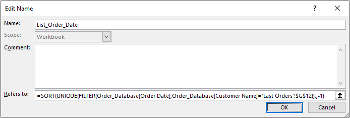
As I mentioned earlier, I am using the dynamic array formulae to make it work, so I might as well go the whole hog.  I also availed myself of other features available in modern Excel.  Let me break the formula into digestible pieces to understand how it works:

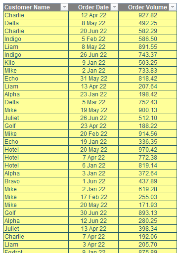
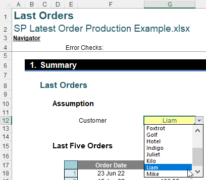
• the FILTER function will get the list of all dates related to the customer selected in cell G12,
• a customer may make multiple orders in a day, so the UNIQUE function will return no duplicates in the list of dates
• therefore, the SORT function will arrange this list based upon descending order (as seeing the most recent order first probably makes the most sense).  This why minus one [-1] is the final argument, ie to ensure the order is descending.

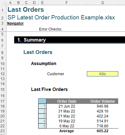
Step 2: Get the list of last five order dates using the INDEX function

Given the List_Order_Date, the cells F18:F22 may be filled using the INDEX function.  In case the list of historical order date related to the customer is less than five [5], the formula should return a blank, viz.

=IFERROR(INDEX(List_Order_Date,E18),"")

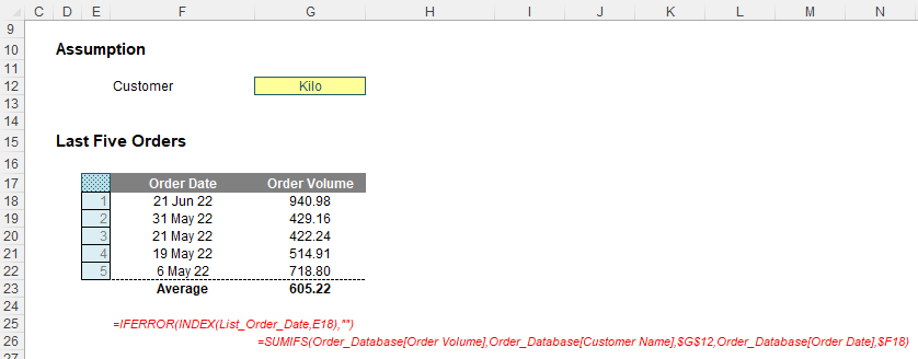
Hence, the order volume can be calculated using the SUMIFS function:

=SUMIFS(Order_Database[Order Volume],Order_Database[Customer Name],$G$12,Order_Database[Order Date],$F18)

You can take a look at the suggested solution using the associated Excel file.