Consider the following example:
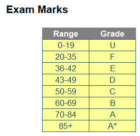
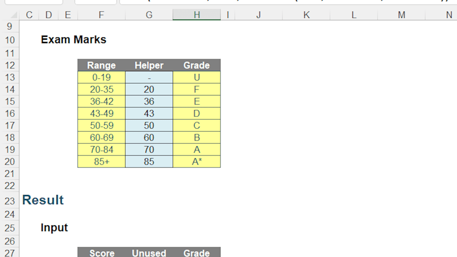
Imagine you are marking an exam, scoring candidates marks out of 100. Any score of 85 or above gains an “A*” grade, a score between 70 and below 85 (84 for simplicity) rates an “A”, a score between 60 and under 70 scores a “B”, and so on.
There is a problem here. The scores in the Range column are viewed as text by Excel, but the scores are numerical. How do I explain to Excel that the numerical value of 57 is in the text range “50-59”? It’s simple to us, but Excel requires assistance. Therefore, we need to address two connected issues:
- We need to convert the text ranges into a numerical register that may be used as a grading barometer
- We also need to decide on which Excel lookup function (given there are so many) is best placed to return the required grade.
Clearly, I need to deal with the first issue, er, first, so let’s start there. I note the scores are in ascending value. Therefore, I can just use the first value in the range to derive the “bucket”, as Microsoft likes to call these bands / ranges of values.
In Power Query, it’s trivial to return the first numerical value (there is a button you can simply click), but I am going to assume we wish to achieve this formulaically in Excel, so I may amend the ranges in real time without needing to hit a ‘Refresh’ button. Thus, I proceed as follows, beginning with a “Helper” column in my table, viz.
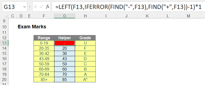
=LEFT(F13,IFERROR(FIND("-",F13),FIND("+",F13))-1)*1
Not my longest calculation ever by any means, but it still needs explaining. It all centres around the FIND function:
FIND("-",F13)
This formula looks for the character position of the hyphen (“-“) in cell F13. In the text string “0-19” (the contents of cell F13), the hyphen is clearly the third character in the text string, so FIND("-",F13) will return the value three [3].
If there is no hyphen, the error message #VALUE! is returned instead. Hence, we “wrap” this formula in an IFERROR expression as follows:
IFERROR(FIND("-",F13),FIND("+",F13))
IFERROR evaluates FIND("-",F13). If it returns a numerical value, that’s fine; if it returns an error, it instead searches for a plus (“+”) symbol in the same cell:
FIND("+",F13)
This is required because of the value in cell F20, i.e. “85+”. Here, FIND("-",F20) would return #VALUE!, but FIND("+",F20) – the formula to calculate if the primary calculation results in an error – would return three [3], as the plus symbol is the third character in this text string.
Therefore, the formula
=LEFT(F13,IFERROR(FIND("-",F13),FIND("+",F13))-1)
will return the text equivalent of the first number in the range for all buckets. For example, in row 20, IFERROR(FIND("-",F13),FIND("+",F13)) returns three [3], so the formula resolves to
=LEFT(F20, 3 – 1)
which would return the two “left-most” characters in the text string “85+”, i.e. “85”. However, this would not be a numerical value, so multiplying by one [1] converts these text strings into numerical values, hence the final formula
=LEFT(F13,IFERROR(FIND("-",F13),FIND("+",F13))-1)*1
This has now addressed our first issue. We now have a numerical register (a list of values in increasing order) we may use to lookup our students’ marks. I now need to consider which function to use to lookup the data.
As with all things in Excel, simplest is bestest. Yes, we have VLOOKUP, HLOOKUP, INDEX MATCH, OFFSET MATCH, SUMIF, SUMIFS, SUMPRODUCT, XLOOKUP et al, but whenever you have data in ascending order in a spreadsheet, your simplest, most reliable function to use is nothing more than the extremely humble LOOKUP function.
LOOKUP Reminder
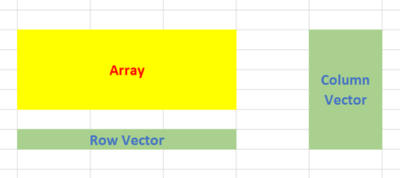
LOOKUP has two forms: an array form and a vector form. Let me explain the jargon:
- an array is a collection of cells consisting of at least two rows and at least two columns
- a vector is a collection of cells across just one row (row vector) or down just one column (column vector).
The diagram should be self-explanatory:
The array form of LOOKUP looks in the first row or column of an array for the specified value and returns a value from the same position in the last row or column of the same array:
LOOKUP(lookup_value, array)
where:
- lookup_value is the value that LOOKUP searches for in an array. The lookup_value argument can be a number, text, a logical value or a name or reference that refers to a value
- array is the range of cells that contains text, numbers or logical values that you want to compare with lookup_value.
The array form of LOOKUP is very similar to the HLOOKUP and VLOOKUP functions. The difference is that HLOOKUP searches for the value of lookup_value in the first row, VLOOKUP searches in the first column, and LOOKUP searches according to the dimensions of array.
If the array covers an area that is wider than it is tall (i.e. it has more columns than rows), LOOKUP searches for the value of lookup_value in the first row and returns the result from the last row. Otherwise, LOOKUP searches for the value of lookup_value in the first column and returns the result from the last column instead. This is why it is dangerous to use and it is usually safer to adopt its sibling variant, the vector form instead:
LOOKUP(lookup_value, lookup_vector, [result_vector])
The LOOKUP function vector form syntax has the following arguments:
- lookup_value is the value that LOOKUP searches for in the first vector
- lookup_vector is the range that contains only one row or one column
- [result_vector] is optional – if ignored, lookup_vector is used – this is the where the result will come from and must contain the same number of cells as the lookup_vector.
Like the default versions of HLOOKUP and VLOOKUP, lookup_value must be located in a range of ascending values, i.e. where each value is greater than or equal to the one before. If this rule is followed, LOOKUP will return the value occurring to the final occurrence of the lookup_value (whereas MATCH would return the first occurrence).
Returning to the Range Lookup
Given our lookup data is in ascending order, we have remarkably little left to do, to find our corresponding grade. LOOKUP in vector form works very well with our Helper column:
My formula in cell H28 is given by
=IF(F28<G13,H13,LOOKUP(F28,G13:G20,H13:H20))
LOOKUP(F28,G13:G20,H13:H20) finds the largest value less than or equal to F28 (87 in the graphic) in the cell range G13:G20, which consists of the values 0, 20, 36, 43, 50, 60, 70 and 85. The largest value less than or equal to 87 is 85. It then looks for the corresponding value in the cell range H13:H20 (which would be the grades), to return the corresponding Grade of A*.
The IF(F28<G13,H13,… statement is simply used to ensure that if the score in cell F28 is less than zero (the value in cell G13, and certainly not a good exam result!), the bottom grade of U (cell H13) is used instead. Since the list is in ascending order, we know for certain that the value in cell G13 represents the lowest value in the cell range G13:G20.
Word to the Wise
Looking up data in ranges is a common problem with a relatively simple solution. You just need to step out the requirement by converting the range to a numerical value that may be used for comparisons and then using an appropriate lookup function. Always aim to get your lookup data into a logical, sequential order. If you achieve this, simple, staid and stolid functions such as LOOKUP can be readily applied by modellers and easily understood by end users alike.