Advanced conditional formatting – part 3: the horror of peril sensitivity

Introduction

The conditional formatting feature in Excel can be used very simply, with just a few clicks required to highlight significant cells or to apply one of three types of graphical format to a range of cells. However, taking the time to explore the capabilities of conditional formatting in a bit more detail can help you to extend what you can achieve and ensure that your formatting looks exactly how you want it to.
In this third and final part of this series we will look at managing existing rules, including multiple rules applied to the same cells, and at how to use conditional formatting in practical situations such as PivotTables and Power Query output tables.

Managing rules

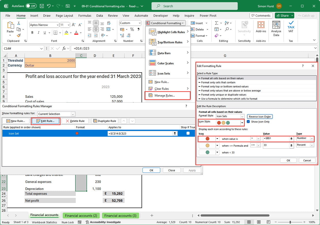
At the bottom of the Conditional Formatting dropdown, a Manage Rules… option allows you to create New Rules, Edit existing rules, Delete and Duplicate rules and to change the order in which rules are applied. We will use an example based on the red highlight circles we created at the end of the previous article:

This method relies on using a version of Excel that allows each icon to be selected individually. For earlier versions a different technique would be required. We could set the top Icon to be displayed in the same way, using a threshold as shown above, but we could add a second rule to the same set of cells that caused other rules not to be applied.

Here, we have used the Conditional Formatting dropdown, Manage Rules… option to open the Conditional Formatting Rules Manager. This displays any existing rules for the selected cells. We have selected our Icon Set rule and clicked on the Edit Rule… button. We have then chosen the traffic lights Icon Style to reset our three icons whilst still using our threshold value rule for the top icon:

Although we will still see our red highlight circles, we will also see amber and green circles where the threshold is not met. To avoid this, we are going to use the New Rule… button to add a rule:

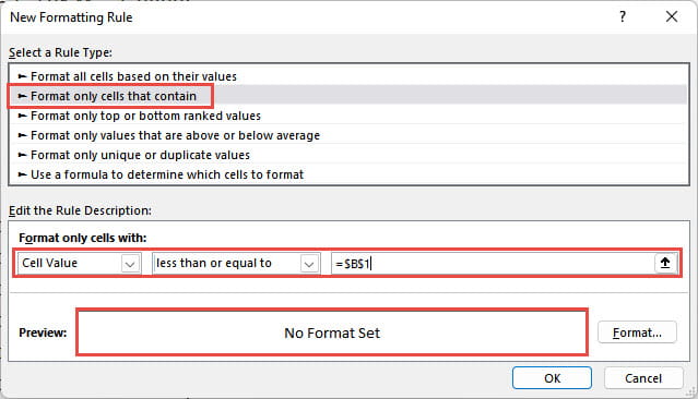
We have used the Rule Type: ‘Format only cells that contain’ and chosen to Format only cells with a Cell Value less than or equal to our threshold cell value, so all the cells that don’t match the criteria of the top of the Icon Sets in our existing rule. Initially, we haven’t set any format for our new rule. With the new rule set up, it makes no difference to how our icons are displayed:

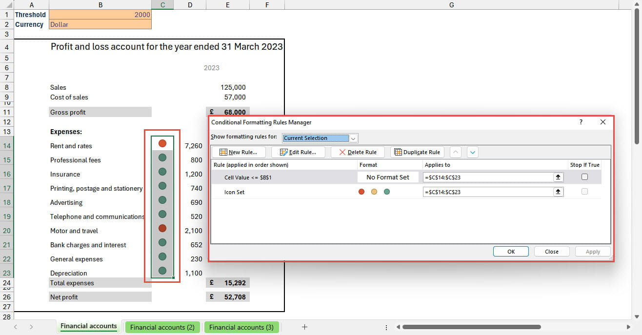
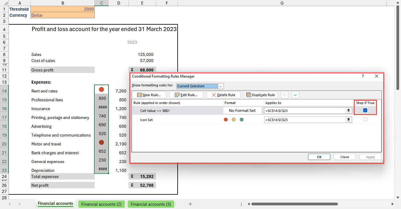
This is because both of our rules will be applied, so for values below our threshold our new rule and our Icon Set rule will be applied giving us the green and amber circles we want to get rid of. To avoid this, we can use the ‘Stop If True’ checkbox for our new rule:

One step forward…

As you can see, we have stopped the Icon Set rule from applying for values below the threshold, but this also means that the Show Icon Only setting isn’t applied, leading the values themselves to appear. There are different ways to address this, but we could change the formatting of our Cell Value rule to use a white font on a white background or just change the normal formatting of the cells to white on white.

Hiding values by using white on white or black on black is generally a bad idea. Not only can it be very confusing for a user, it can also be used to mislead and, although it seems to have hidden the values or formulas, they still show up in the formula bar when the cell is selected and it only takes a mouse click to reset the formatting and display the apparently secret values.

If you think this sounds a little far-fetched, it’s worth looking through the European Spreadsheet Risk Interest Group’s (EuSPRIG) horror stories page for the Westpac entry:

“Westpac was forced to halt trading on its shares and deliver its annual profit briefing a day early after it accidentally sent its results by email to research analysts. Details of the $2.818 billion record profit result for the 12 months to September 30, were embedded in a template of last year’s results and were accessible with minor manipulation of the spreadsheet. (Some reports indicated an employee had thought that a black cell background fill would hide black text.)”

Rule priority

Whilst we are looking at multiple rules, it’s worth considering how the order of the rules in the Rules Manager affects which conditional formats are applied, when the conditional formats themselves are mutually exclusive. The inclusion of up and down arrows to change the position of the rules in the list suggests that the order is significant, and you might think that the rules would be applied from the top down. This simple example shows that this is not true:

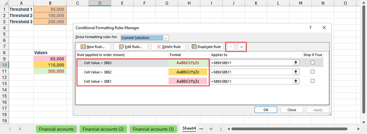
Given that all three of our values meet the criteria of our bottom rule and they all apply a fill colour, if the rules were applied from top to bottom, you would expect all cells to use the bottom rule format. In fact, the order is only important when more than one criterion is TRUE and, when this is the case, the rule higher in the list overrides any other TRUE rule that applies the same type of format. 60,000 only passes the third rule in the list, so this is the rule that is used and the other two are not considered. For 110,000 the bottom two rules are TRUE so the higher rule in the list is applied (amber). For 300,000 all rules are TRUE so the highest rule in the list (green) is used.

Conditional formatting with PivotTables

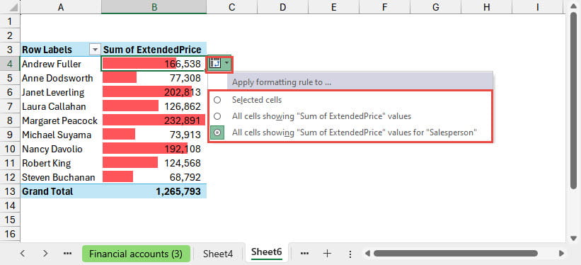
Prior to the introduction of Excel 2007, it was very difficult to use conditional formatting with a PivotTable as the formatting only applied to cells rather than PivotTable areas so, when the PivotTable dimensions changed, the formatting was no longer applied to the correct cells. Excel 2007 changed this and allowed formatting to be extended to a particular area of the PivotTable. Here, we have applied a Solid Fill Red Data Bar to a single PivotTable cell. Given that Data Bars show the comparative values of multiple cells, this seems an odd thing to do, but a Formatting Options icon will appear and let us apply the format to All cells showing “Sum of ExtendedPrice” values or All cells showing “Sum of ExtendedPrice” values for “Salesperson”. We have used the latter option in order to exclude the Grand Total value from the comparison which would dwarf all the other data bars:

Conditional formatting with Excel Tables, including Power Query output Tables

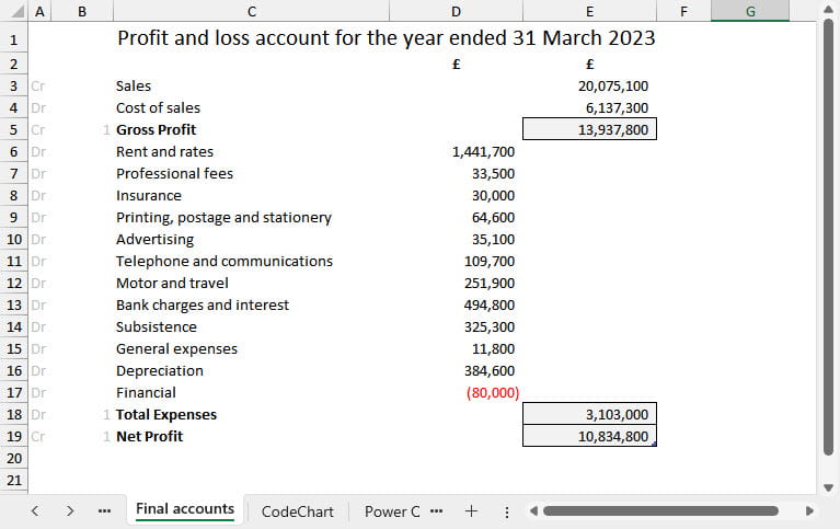
It is possible to apply conditional formatting to entire Table columns whether they are part of a standalone Excel Table or an Excel Table generated by Power Query. In both cases, as the Table expands, the conditional formatting will automatically be extended to any new cells. This makes it possible for Power Query to generate, for example, a formatted set of accounts as an output Table, with hidden ‘helper’ columns used to format negative and positive values, and totals, using conditional formatting:

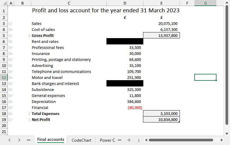
Peril sensitivity

Those familiar with the Hitchhiker’s Guide to the Galaxy might remember:
“Joo Janta 200 Super-Chromatic Peril Sensitive Sunglasses [which] have been specially designed to help people develop a relaxed attitude to danger. At the first hint of trouble, they turn totally black and thus prevent you from seeing anything that might alarm you.”
Clearly, conditional formatting would be an ideal way to apply the same principle to Excel spreadsheets automatically (noting the comments about invisibility and horror stories above):

Conclusion

For more articles on conditional formatting, search the ICAEW Excel Community article archive: