Allowing for Errors with SUMPRODUCT

With the advent of dynamic array formulae, eta lambdas, et al, everyone has been delighting in telling me that the SUMPRODUCT function is on its last legs. I think that might have something to do with the name of my company, but I shall assure you there is definitely life in the old dog still.

If you don’t have Office 365, SUMPRODUCT is certainly useful for dealing with data calculations in Excel. Don’t give up on it just yet!

Whilst a highly versatile function, there does appear to be the odd occasion when it appears to struggle. Consider the following example:

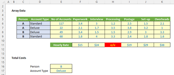
Imagine you wished to cross-multiply all costs that meet certain criteria. The criteria (Business and Account Type) are provided in cells C6:C9 and D6:D9, with the number of accounts in cells E6:E9. The hours required for the various processes per account type and business are in cells F6:K9 with the hourly rates by process in cells F11:K11.

In summary, if all costs were calculated, you’d need to cross multiply all of the cells, e.g. (117 x 3.4 x $15) + (117 x 3.0 x $24) + (117 x… etc.

But it’s harder than that. Firstly, I only want to include costs that meet certain criteria (Business “B” and account type “Deluxe”, say) and secondly, I decided to make one of the hourly rates “n/a”.

In one cell, without adding any helper rows or columns or using different data or VBA, I could write the following horror formula:

The problem with this solution is (a) it won’t scale (e.g. add extra accounts or processes) and (b) even Einstein would struggle to follow it (especially as he’s otherwise occupied these days, starring in things like Oppenheimer).

Here’s my suggested solution:

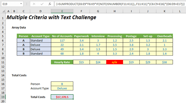
{=SUMPRODUCT(E6:E9*F6:K9*IF(NOT(ISNUMBER(F11:K11)),,F11:K11)*(C6:C9=E16)*(D6:D9=E17))}

Simple!

If that’s all you need to know, glad to be of help. But I’m thinking you might want an explanation.

Let me introduce our namesake, the humble SUMPRODUCT function. At first glance, SUMPRODUCT(vector1, vector2, ...) appears quite ordinary. However, before showing an example, though, look at the syntax carefully:

• a vector for Excel purposes is a collection of cells either one column wide or one row deep. For example, A1:A5 is a column vector, A1:E1 is a row vector, cell A1 is a unit vector and the range A1:E5 is not a vector (it is actually an array, but more on that later). The ranges must be contiguous; and
• this basis functionality uses the comma delimiter (,) to separate the arguments (vectors). Unlike most Excel functions, it is possible to use other delimiters, but this will be revisited shortly below.

To illustrate, let’s consider the following sales report:

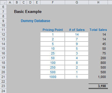
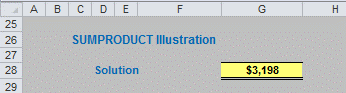
The sales in column H are simply the product of columns F and G, e.g. the formula in cell H12 is simply =F12*G12. Then, to calculate the entire amount cell H23 sums column H. This could all be performed much quicker using the following formula:

=SUMPRODUCT(F12:F21,G12:G21)

i.e. SUMPRODUCT does exactly what it says on the tin: it sums the individual products.

Where SUMPRODUCT comes into its own is when dealing with multiple criteria. This is done by considering the properties of TRUE and FALSE in Excel, namely:

• TRUE*number = number (e.g. TRUE*7 = 7); and
• FALSE*number = 0 (e.g. FALSE*7=0).

Consider the following example:

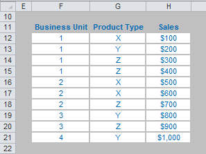
we can test columns F and G to check whether they equal our required values. SUMPRODUCT could be used as follows to sum only sales made by Business Unit 1 for Product Z, viz.

=SUMPRODUCT((F12:F21=1)*(G12:G21=“Z”)*H12:H21).

For the purposes of this calculation, (F12:F21=1) replaces the contents of cells F12:F21 with either TRUE or FALSE depending on whether the value contained in each cell equals 1 or not. The brackets are required to force Excel to compute this first before cross-multiplying.

Similarly, (G12:G21=“Z”) replaces the contents of cells G12:G21 with either TRUE or FALSE depending on whether the value “Z” is contained in each cell.

Therefore, the only time cells H12:H21 will be summed is when the corresponding cell in the arrays F12:F21 and G12:G21 are both TRUE, then you will get TRUE*TRUE*number, which equals the said number.

You should note that this uses the * delimiter rather than the comma, analogous to TRUE*number, etc. If you were to use the comma delimiter instead, the syntax would have to be modified thus:

=SUMPRODUCT(--(F12:F21=1),--(G12:G21=“Z”),H12:H21).

Minus minus? The first negation in front of the brackets converts the array of TRUEs and FALSEs to numbers, albeit substituting -1 for TRUE and 0 for FALSE. The second minus sign negates these numbers so that TRUE is effectively 1, rather than -1, whilst FALSE remains equals to zero. This variant often confuses end users which is why I recommend the first version described above.

You can get more and more sophisticated:

So far, I have only considered SUMPRODUCT with vector ranges. Using the multiplication delimiter (*), it is possible to use SUMPRODUCT with arrays (an array is a range of cells consisting of both more than one row and more than one column).

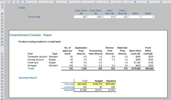
In the above example, SUMPRODUCT has been used in its elementary form in cells I36:N36. For example, the formula in cell I36 is:

=SUMPRODUCT($H$32:$H$35,I$32:I$35)

and this has then been copied across to the rest of the cells.

To calculate the total costs of this retail bank example, this could be calculated as:

=SUMPRODUCT($I$36:$N$36,$I$21:$N$21)

However, the formula in cell I41 appears more – and unnecessarily – complicated:

=SUMPRODUCT($H$32:$H$35*$I$32:$N$35*$I$21:$N$21)

The use of the multiplication delimiter is deliberate (the formula will not work if the delimiters were to become commas instead). It should be noted that this last formula is essentially

=SUMPRODUCT(Column_Vector*Array*Row_Vector)

where the number of rows in the Column_Vector must equal the number of rows in the Array, and also the number of columns in the Array must equal the number of columns in the Row_Vector.

The reason for this extended version of the formula is in order to divide the costs between Budget and Standard costs in my example. For example, the formula in cell J41 becomes:

=SUMPRODUCT($H$32:$H$35*$I$32:$N$35*$I$21:$N$21*($G$32:$G$35=J$40))

i.e. the formula is now of the form

=SUMPRODUCT(Column_Vector*Array*Row_Vector*Condition)

where Condition uses similar logic to the TRUE / FALSE examples detailed earlier. This is a powerful concept – and now you can see how this will answer our question.

Using the above syntax, I can try the following:

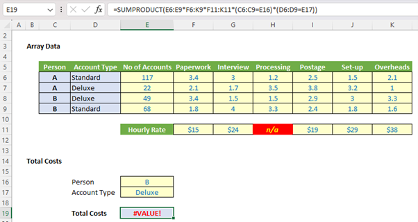
Unfortunately, using the syntax described above, I obtain

=SUMPRODUCT(E6:E9*F6:K9*F11:K11*(C6:C9=E16)*(D6:D9=E17))

But that gives me #VALUE! That’s because cell H11 contains the text “n/a”. SUMPRODUCT doesn’t like text. SUMIFS does. See the difference in this next example?

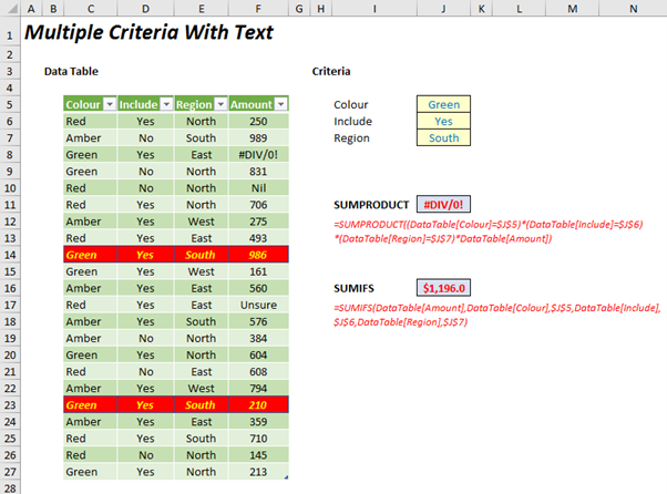
Do you see SUMIFS works even though I have failed to explain either the syntax or the formula? This is because SUMIFS only works on vectors and my problem – deliberately – uses arrays. My solution does employ SUMPRODUCT but in an unusual way. Did you notice “n/a” was highlighted bold italic yellow on red in the original Excel file?

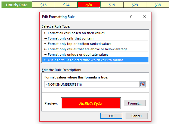
That’s because I used conditional formatting. It highlights the cell accordingly if

=NOT(ISNUMBER(F$11))

is TRUE. ISNUMBER determines if a cell or value is a number; NOT converts TRUE to FALSE and vice versa. Therefore, a cell is highlighted if it does not contain a number.

Now consider my solution. It expands on my first attempt for the solution as follows:

{=SUMPRODUCT(E6:E9*F6:K9*IF(NOT(ISNUMBER(F11:K11)),,F11:K11)*(C6:C9=E16)*(D6:D9=E17))}

Note that this formula replaces F11:K11 with IF(NOT(ISNUMBER(F11:K11)),,F11:K11). That means text is treated as zero – a nice workaround trick which makes the SUMPRODUCT syntax work provided that the formula has been entered as an array (CTRL + SHIFT + ENTER to get the ‘curly brackets’ formally known as braces). (This is a syntax requirement for Excel other than Excel 365.)

As I said, simple!

Have a great festive break and a happy new year.