Advanced Data Validation – part 4: optimise data input dropdown lists with dynamic arrays

Excel’s Data Validation feature can be very useful in helping to ensure that users enter the correct information into input cells. In this series we will look at some of the less obvious capabilities of the feature. Part 1 covered the basics of Data Validation before moving on to the use of formulas, functions and cell references to calculate the criteria values used as part of the standard ‘Allow’ options. Part 2 looked at the use of the Custom option to create criteria based solely on an Excel formula, including using the COUNTIFS() function to create a Data Validation setting to reject duplicate items. Part 3 looked at restricting user entries to items included in a list of values or a range of cells.

As part of our initial look at lists, we covered a recently introduced enhancement that adds AutoComplete to Data Validation lists. This enhancement also automatically ignores duplicate items in the source list. This time we will look at an alternative method of removing duplicates and also tailoring a list to match our exact requirements.

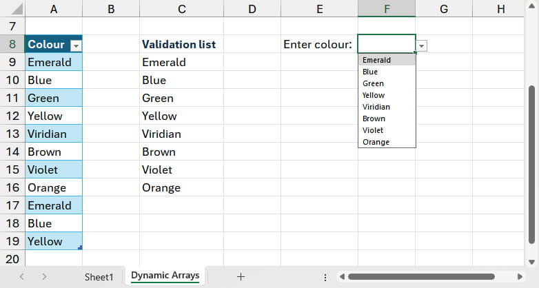
If our original source list isn’t quite in the format that we want it to be in for our Data Validation dropdown list, we will need to process it in some way. We will also probably need our processed list to update automatically as the original source list changes, including expanding and contracting as items are added or removed. The easiest way to achieve this, without the need to use automation code or a refresh operation, is to use a Dynamic Array formula. If you don’t have access to the Data Validation enhancement that automatically excludes duplicate entries from a list, you can use the UNIQUE() Dynamic Array function instead:

=UNIQUE(Colours[Colour])

Here, we have entered our Dynamic Array formula in cell C9 to create our unique list and then based our Data Validation source list on the range of cells C9:C16:

Although this works with the current source list entries, and will reflect changes in the existing entries, if we were to add more items, our Data Validation list will still just refer to the original range:

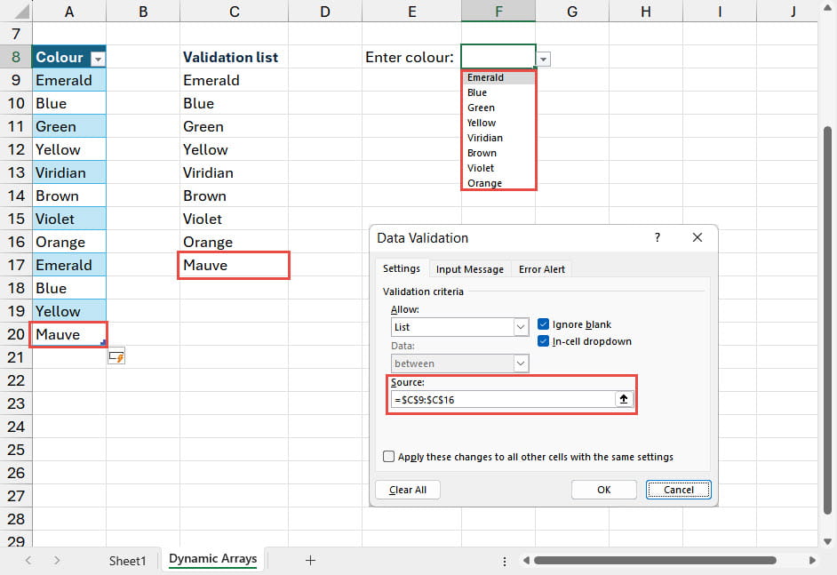
One of the drawbacks of using Dynamic Arrays is that the resulting range of cells cannot be created as an Excel Table, which means the usual methods of allowing Excel to adapt to the expansion or contraction of the original list aren’t available. However, the # operator allows an Excel formula to refer to the result of a Dynamic Array formula without the need to use a Table. Here, in our Data Validation source, we have referred to just the cell that contains our Dynamic Array formula and added the # as a suffix:

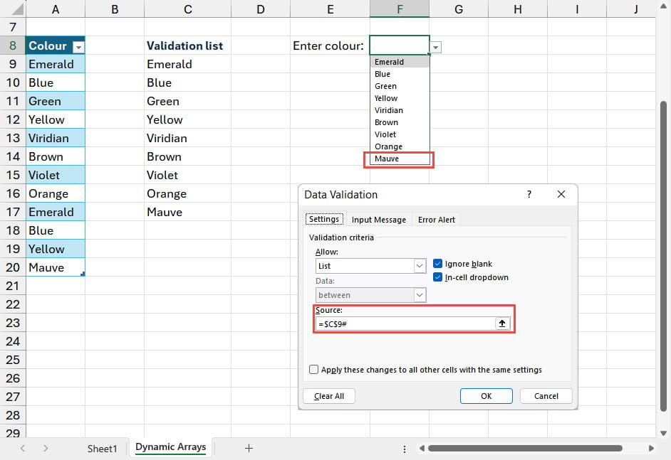
As you can see, our Data Validation dropdown list now adapts to include the additional entry in the original source list.
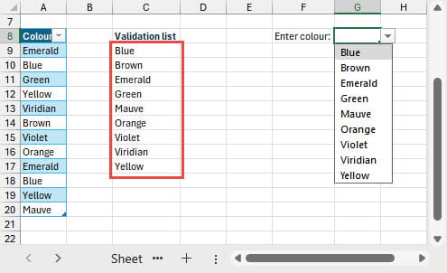
Particularly if your version of Excel doesn’t support AutoComplete, it can be helpful to sort your dropdown list items to help make it easier for users to find the item they want to use. The SORT() Dynamic Array function will do this and can be combined with the UNIQUE() function:

=SORT(UNIQUE(Colours[Colour]))

There is a FILTER() Dynamic Array function that allows an array to be filtered to show only items where a formula evaluates to TRUE. Here, we have expanded our example to show paint Finish as well as Colour. We want to allow the user to select a paint finish and a colour, but we want to restrict the colours dropdown list to only include colours available for that finish:

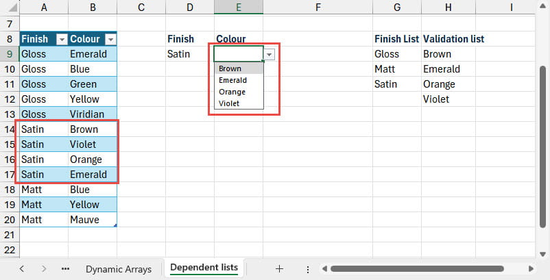
We create the list to use as our Finish Data Validation list source using the formula in G9:

=SORT(UNIQUE(Colours[Finish]))

In H9 we use the FILTER() function to restrict the items in our list to those where the Finish column row values match the entry we have chosen in our Data Validation cell D9:

=SORT(UNIQUE(CHOOSECOLS(FILTER(Colours,Colours[Finish]=D9),2)))

We use SORT() and UNIQUE() as before, but we also use the FILTER() function to only include rows where the entry in the Finish column of our table matches the value selected in cell D9. We only want to return our Colours column, so we use the Dynamic Array CHOOSECOLS() function to select column 2 of our table.

• For more articles on Data Validation, search the ICAEW Excel Community article archive