
It’s time to round out our lookup functions, but not before we ask the following question: do you choose to use CHOOSE? This function uses index_number to return a value from the list of value arguments. CHOOSE may be used to select one of up to 254 values based on the index number (index_number). For example, if value1 through value7 are the days of the week, CHOOSE returns one of the days when a number between 1 and 7 is used as index_number.
The CHOOSE function employs the following syntax to operate:
CHOOSE(index_number, value1, [value2])
We now have a list of posts with additional information about the series they belong to and the author, and we can click on the Link hyperlink to open that article in a browser:
The CHOOSE function has the following arguments:
- index_number: this is required and is used to specify which value argument is to be selected. The argument index_number must be a number between 1 and 254, or a formula or reference to a cell containing a number between 1 and 254.
- if index_number is 1, CHOOSE returns value1; if it is 2, CHOOSE returns value2; and so on
- if index_number is less than 1 or greater than the number of the last value in the list, CHOOSE returns the #VALUE! error value
- if index_number is a fraction, it is truncated to the lowest integer before being used.
- value1, value2, ...: value 1 is required, but subsequent values are optional. There may be between 1 and 254 value arguments from which CHOOSE selects a value or an action to perform based on index_number. The arguments can be numbers, cell references, defined names, formulas, functions, or text.
It should be further noted that:
- if index_number is an array, every value is evaluated when CHOOSE is evaluated
- the value arguments to CHOOSE can be range references as well as single values.
For example, the formula:
=SUM(CHOOSE(2, A1:A10, B1:B10, C1:C10))
evaluates to:
=SUM(B1:B10)
The CHOOSE function is evaluated first, returning the reference B1:B10. The SUM function is then evaluated using B1:B10, the result of the CHOOSE function, as its argument. A similar idea is also expressed by the formula
Certainly it is a function used in modelling, but perhaps it is not used as regularly as some others. This is useful for non-contiguous references:

Just so that we are clear on jargon: a non-contiguous range (with reference to Excel) means a range that cannot be highlighted with the mouse alone. In the image above, to highlight the cells coloured you would have to press down the CTRL key as well.
INDEX, LOOKUP, VLOOKUP and HLOOKUP all require contiguous references. They refer to lists, row vectors, column vectors and / or arrays. CHOOSE is different:
=CHOOSE(index_number, value1, [value2]…)
As explained above ,this function allows references to different calculations, workbook / worksheet references, etc. Try to use the function appropriately. For instance, a well-known Excel website proposes the following formula for calculating the US Thanksgiving date. Assuming cell A1 has the year:
=DATE(A1, 11, CHOOSE(WEEKDAY(DATE(A1, 11, 1)), 26, 25, 24, 23, 22, 28, 27))
To understand this formula, note that DATE(year, month, day) returns a date and WEEKDAY(date) returns a number 1 (Sunday) through 7 (Saturday). But doesn’t this formula look horrible? It is full of hard code and it contains an unnecessary number of arguments. The formula could exclude CHOOSE viz.
=DATE(A1, 11, 28 - MOD(WEEKDAY(DATE(A1, 11, 1)) + 1, 7))
Now let me be clear here. I am not saying this is a simple, transparent formula. Test it. They both provide the same answer. CHOOSE – and plenty of additional hard code – has been used unnecessarily.
That’s not to say there isn’t a time and a place for CHOOSE. It is useful when you need to refer to cells on different worksheets or in other workbooks. Some argue that it is useful when a calculation needs to be computed using different methods, e.g.
=CHOOSE(index_number, calculation1, calculation2, calculation3, calculation4)
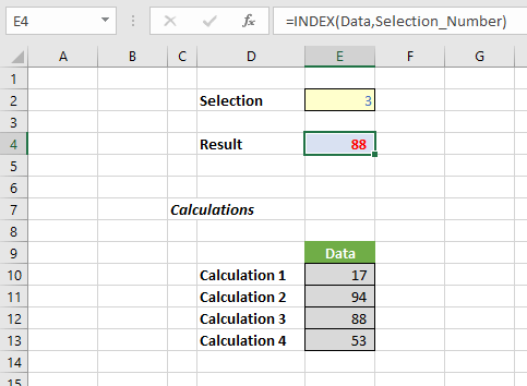
It’s identical, but easier to follow
=INDEX(Data, Selection_Number)
I have taught financial modelling to many gifted analysts over the years and a common mistake made by many is that they build models that are easy to build rather than models that are easy to understand. The end user is the customer. It should be simple to use: taking shortcuts invariably only helps the modeller – and even then, more often than not, shortcuts will backfire.
CHOOSE can lead to opaque models that need to be rebuilt and are often less flexible to use. You have been warned!
Archive and Knowledge Base
This archive of Excel Community content from the ION platform will allow you to read the content of the articles but the functionality on the pages is limited. The ION search box, tags and navigation buttons on the archived pages will not work. Pages will load more slowly than a live website. You may be able to follow links to other articles but if this does not work, please return to the archive search. You can also search our Knowledge Base for access to all articles, new and archived, organised by topic.