What’s so special about “GO TO SPECIAL”?

The basics

“Go To Special” is a function which will find cells within a selection which meet certain criteria, for example finding all the constants, or all the formulae etc.

To use it first select a range of cells then bring up the “Go To Special” menu by pressing F5 then ALT+S (Alternatively you can go to the home tab on the ribbon and click on “Find and Select” and then “Go To Special”.) Then from the menu, select what type of cells you want to go to, and then click OK. Excel will then select the subset of cells from your selection which matched that criteria.

For example, if you want to find certain cells in a range of formulae which have been overtyped with constants, you would select the block of formulae cells, press F5 then ALT+S, then click on the “Constants” option from the menu and click OK.

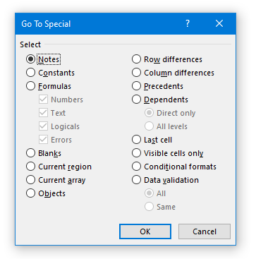
Go To Special Menu:

Features & Applications

There’s so much that this seemingly simple function can do I’ll try to cover each in turn, and include some examples, but I’m sure you’ll also come up with your own use cases as you get to grips with it. I have listed all the functions below in the order they appear on the menu, not necessarily in their order of importance.

Notes

This will find cells which have ‘notes’ attached to them, be aware that this will not identify cells which have ‘comments’ attached. If you do need to find cell comments, then the easiest way to do that is via the Review tab on the ribbon and use the next / previous comment buttons.

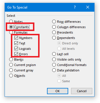
Constants

This is a really helpful function to find constants – and not only constants but different types of constants. Unfortunately, the menu is a bit misleading because it places the check boxes beneath the “Formulas” button, even when you have Constants selected, but rest assured you can check / uncheck different types of constants using the tick boxes and that will work.

In the image below I’d be finding all types of constants, but I only wanted numbers I could untick the text, logical and errors boxes.

As mentioned in the introduction a really good application for this is if you want to find where formulae have been overtyped with hardcoded values in the middle of a calculation block. It’s not good practise to overtype formulae, but, as we all know, sometimes it happens, and this can help find those instances.

Go to Constants

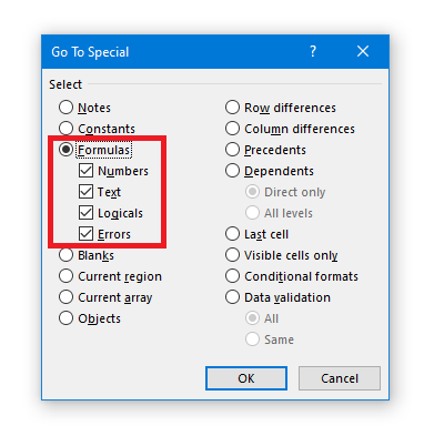
Formulas

Similar to the use for constants it’s also possible to filter to only find formulae which result in numbers, text, logicals (true / false) or errors by using the same tick boxes.

Go to Formulas:

My favourite application is when this is used in conjunction with Copy and Paste to select the cells I want to paste into. For example, if I’m putting together a presentational output sheet which needs gaps between the columns. If I need to update a formula on a particular row then I can change the first column but then how do I update all the other columns, given there are gaps between I can’t just drag it to the right. What I do instead is to select my cell and press CTRL+C to copy it, then highlight the entire row (using SHIFT+SPACE) then press F5, ALT+S to open Go To Special, and select Formulas and click OK. My selection then reduces to just the formula cells on the current row – i.e., it has skipped over the blank cells between columns. I can now press CTRL+V to paste my formulae into all the required columns only, and no matter how many columns I had to update it’s all done in just a few keystrokes.

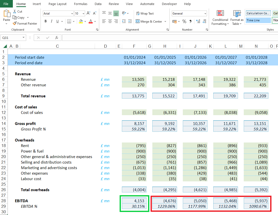
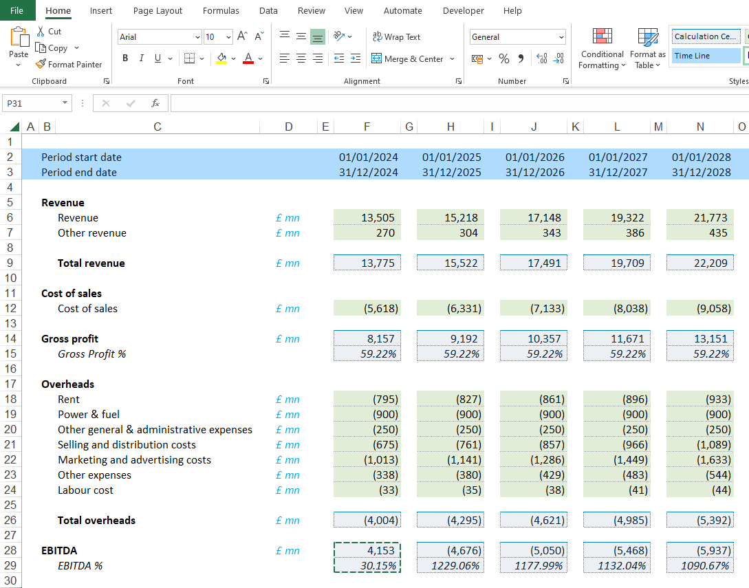
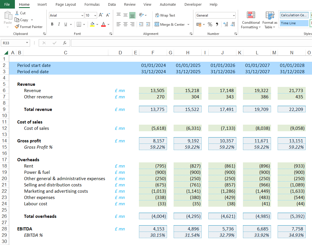
Starting point – In this demo the formulae for EBITDA £ and EBITDA % have been updated in F28:F29 and these formulae need to be updated in all columns across the row.

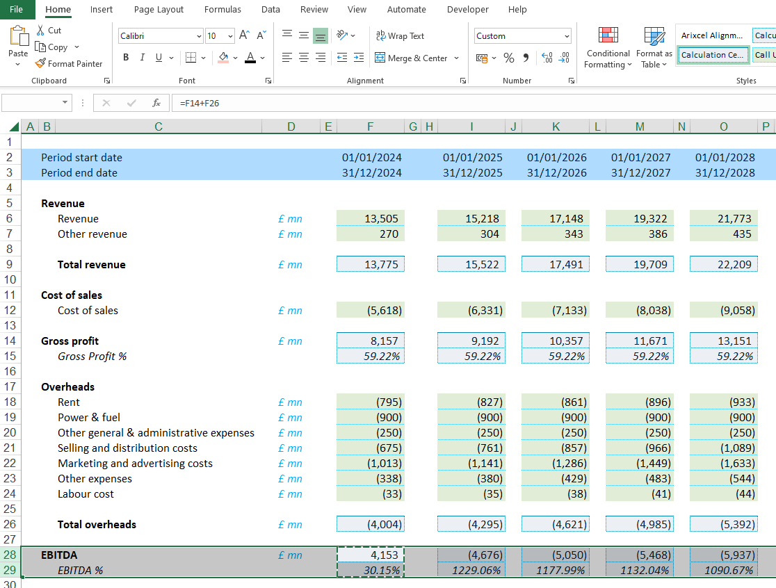
Step 1 – Select the two cells to copy and press CTRL+C to copy them:

Step 2 – Select the other cells in the row

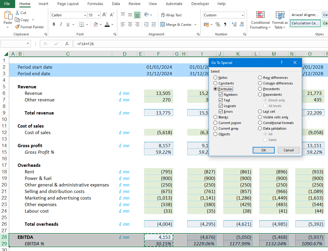
Step 3 – Press F5, ALT+S to open Go To Special and select formulae, then click OK

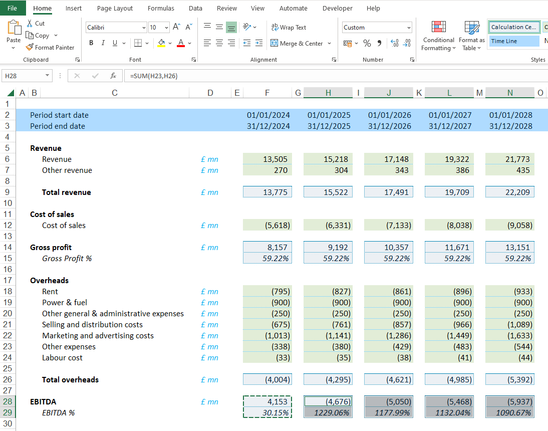
Step 4 – The selection now only picks up the cells which have formulas in them, i.e. it misses out the headings which are constant text, and also skips over the blank cells.

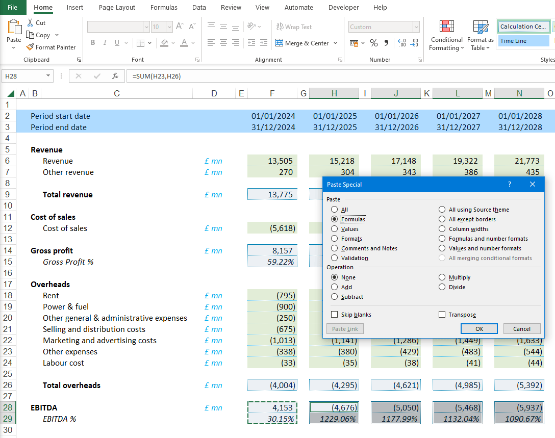
Step 5 – With the formulae cells selected press ALT+E,S to open the Paste Special menu and select paste formulae.

Finished – The formulae have been updated in all the columns:

Blanks

As simple as the description sounds, this one just selects the blank cells in a selection.

An example use case for this might be if you had some data and needed to remove empty rows, you could select a range which covers the first column of the data, then use Go To Special to go to the blank cells, then press CTRL+- (the minus sign) and when prompted select “delete entire row”.

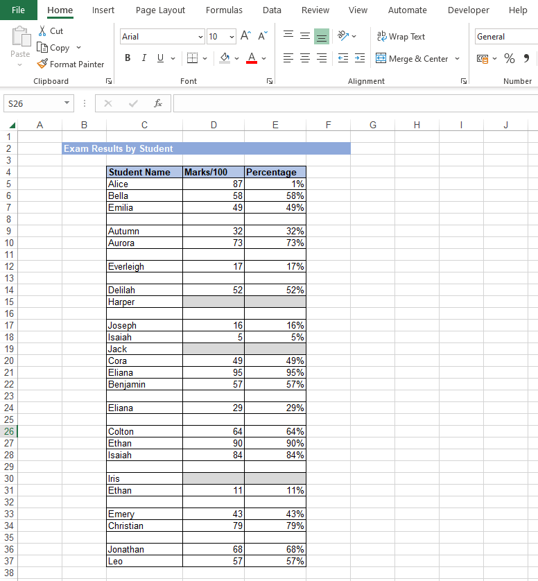
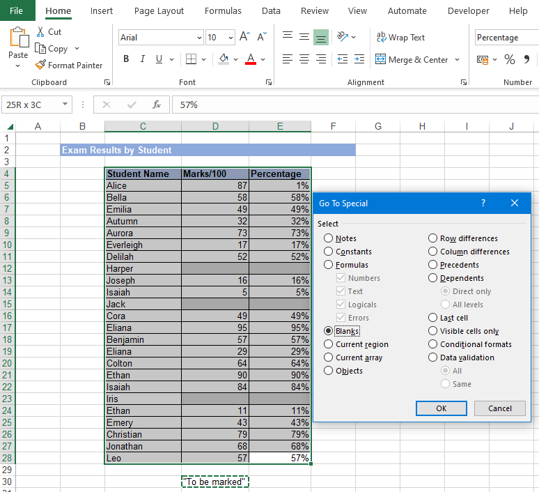
Starting point – In this demo there is a table of student exam results which has rows where some students have been deleted and an empty row remains, and some students where the scope is missing. The blank rows need to be deleted and some default text added in the missing score cells.

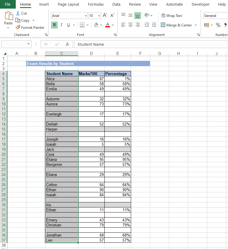
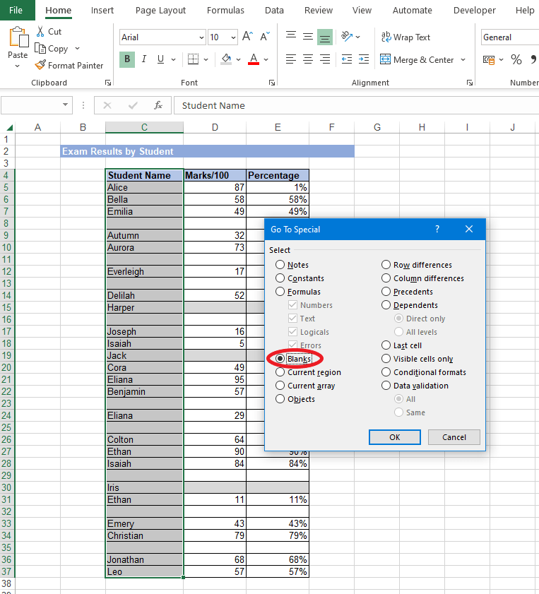
Step 1 - Select the column with the student names and the gaps in it:

Step 2 – Use Go To Special to select the blanks

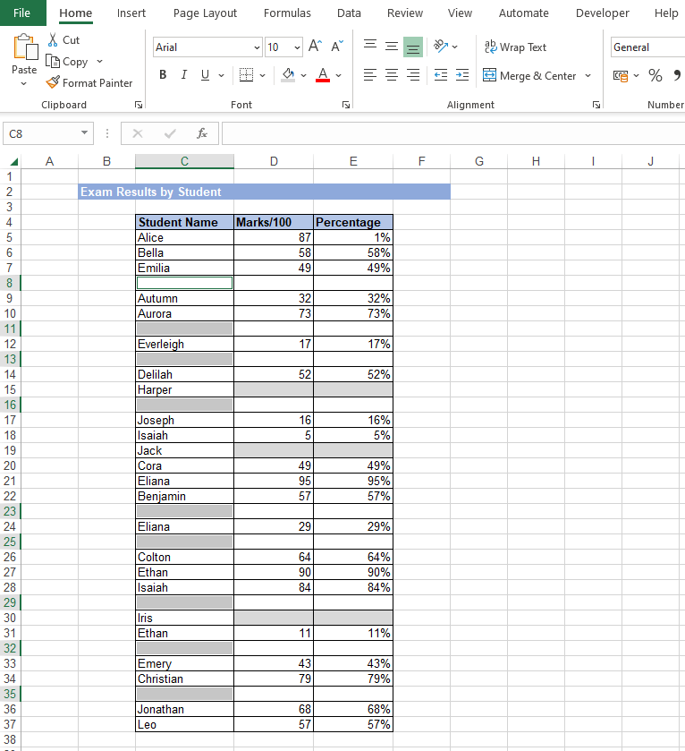
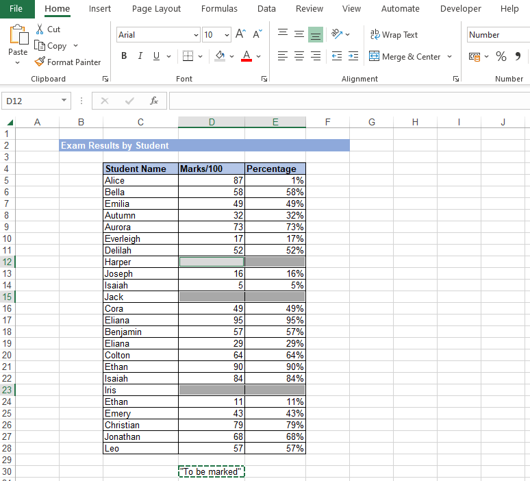
Step 3 – Selection is now on the blank name cells only

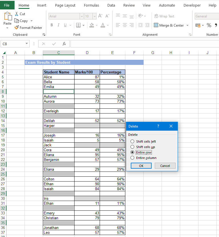
Step 4 – Press CTRL+- (the minus sign) to bring up the delete dialogue box and select entire row

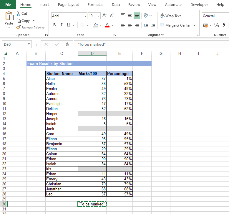
Step 5 – Now the rows are fixed, we need to add default text into the blank score cells. Type “To Be Marked” into a spare cell, select it and press CTRL+C to copy

Step 6 – Select the entire table this time and use Go To Special to select the blank cells

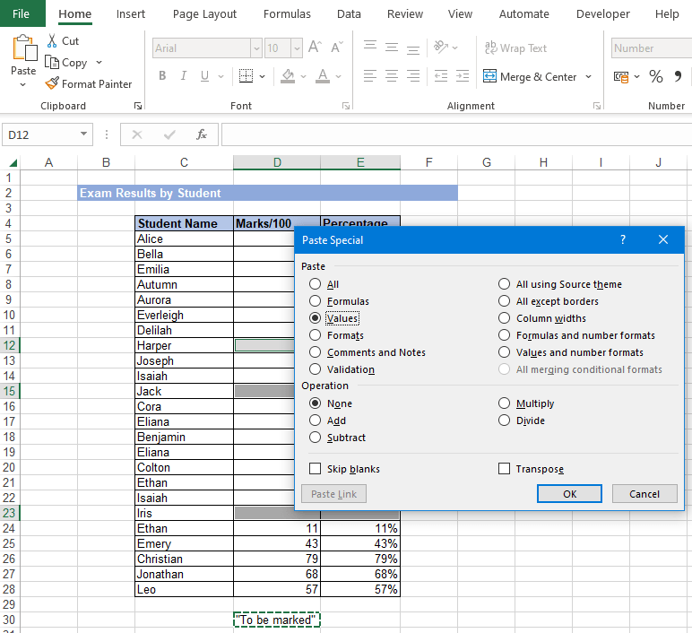
Step 7 – The selection is now on the empty score cells:

Step 8 – Finally use past special to paste the default value to the selected cells:

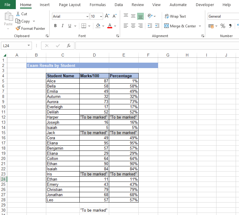
Finished – The blank rows have been removed and default data added to the missing scores:

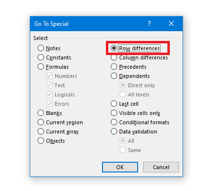
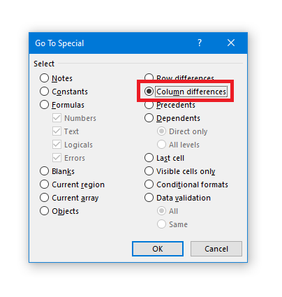
Row or Column differences

This is another really powerful feature which I will cover in more detail in parts 2 and 3 of this blog, but in short it can be used to find formulae cells where the formulae is not the same as the first cell in the selection.

Go to Row Differences

Go to Column Differences

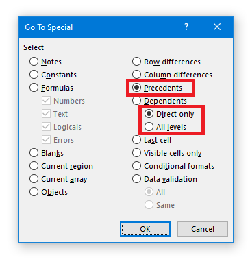
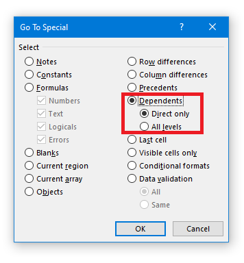
Precedents or  Dependents

This is similar to the formula auditing tool “trace precedents” in so far as it will help to identify the cells which feed into the current cell, but it has a few extra tricks available(!)

Go to Precedents

Go to Dependents

Firstly, it can operate on multiple cells at a time, i.e., you can select a range of cells and use this function to select those cells which are precedents of any of the selected cells – whereas  the formula auditing tool can only trace precedents from the single active cell.

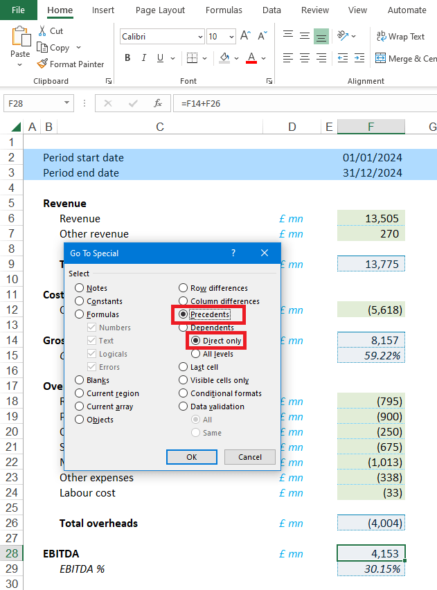
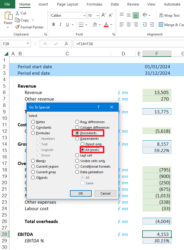
Secondly it can be used to trace all levels, not just one level. I.e., instead of going back to just immediate precedents (one level) you can set to “All levels” in order to select all of the cells which feed into ANY of the selected cells. Using the formula auditing tool, you can only get one level at a time and have to press the button multiple times to trace multiple steps. Note that Go To Special can be made to trace only one level by choosing “Direct only” in the menu. (Note also, similar to the settings for Constants and Formulae, the selection for level appears underneath Dependents but applies to Precedents if that’s what you’ve chosen).

Finally, the Go To Special function actually selects the cells which are precedents, which means you can do something with them (hint – you might want to colour them in…) whereas the formula audit version only shows visual arrows and therefore may not be as helpful.

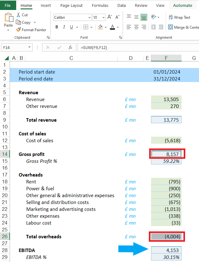
Starting point – In this demo we want to identify which cells flow into the EBITDA £ value in cell F28:

Option 1 – Using the ‘Direct only’ will show the cells which immediately flow into the selected cell, in this case it’s cells F14 and F16 as can be seen in the formula bar also:

Result – The two immediate precedents are selected:

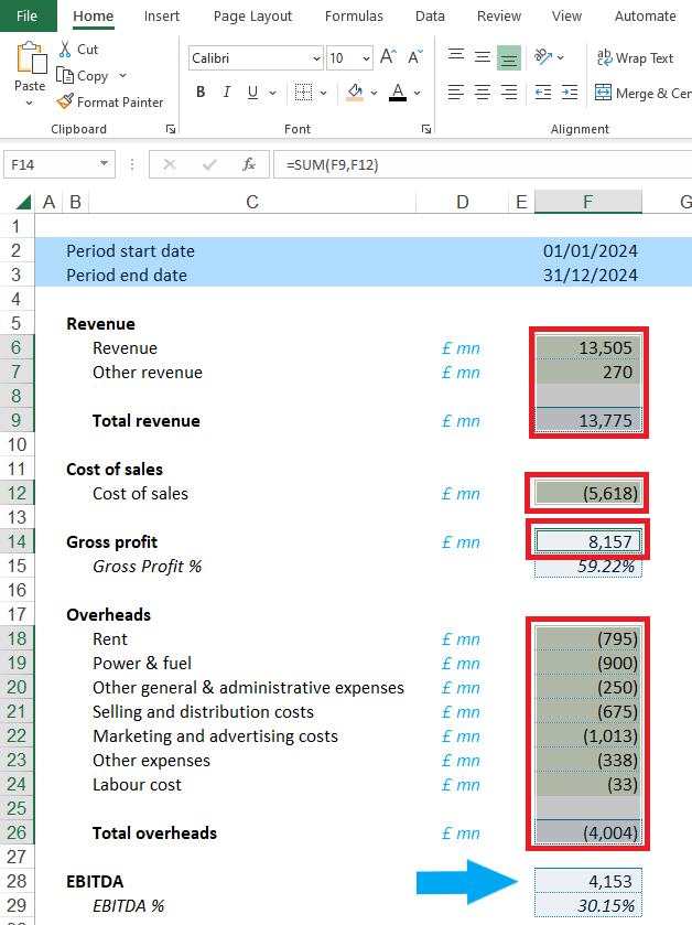
Option 3 – Using the ‘All Levels’ will show all the cells on this sheet which flow into the selected cell, no matter how many other steps are in between:

Result – Not only are the two immediate precedents selected, but also all of the sub totals and figures which feed into EBITDA:

Visible cells only

As the name suggests, this one selects only visible cells. Cells might be hidden due to rows / columns begin hidden or grouped, if you selection crosses a range of hidden cells then those cells are included in the selection however you might not want to interact with them, depending on what you’re doing. For example, using CTRL+D to fill down, or CTRL+V to paste into an area with rows not visible due to being hidden or grouped WILL still write values into those hidden rows. So, using Go To Special visible cells first will then allow you to use CTRL+D or CTRL+V to paste into only the visible rows.

Note, there’s an interesting quirk of Excel that means that CTRL+D and CTRL+V will NOT write into hidden or grouped rows if there is an auto filter applied on the sheet, even if those rows are not part of the filter range(!) So sometimes CTRL+D and CTRL+V will write into hidden cells and sometimes they won’t but using Go To Special visible cells only first will take the guesswork away and reduce the risk of overwriting values unintentionally.

Other functions

The functions for “Objects”, “Current Region”, “Current Array”, “Last cell”, “Conditional formats”, and “Data validation” are self-explanatory so there’s not a lot for me to add(!)

Conclusion