How can “GO TO SPECIAL” help when reviewing logic on a spreadsheet?

Best Practice and Risk Management

This blog is about using Go To Special, but it’s probably helpful to have a quick recap on spreadsheet best practice – more information is available in ICAEW’s 20 Principles of Good Spreadsheet Practice. But the key I want to focus on here is the use of consistent formulae in a block. This means writing a single formulae which can be dragged across all the rows or columns in a block. If a spreadsheet has different formulae across a timeline, or down a column in a table of data, then there is a risk that things would go wrong if the spreadsheet is updated.

For example, it might be tempting to amend a formula to cope with an “exception” which needs to happen only in a certain month or on a certain row of data. The problem comes if the model is updated and the column or row with the exception changes in the source data, but the formulae are not updated – this will mean that the inconsistent formulae now sit in the wrong column or row. Likewise another issue would arise if an update was required to the general logic and the first cell is updated and it’s then dragged across the whole range by a well-meaning model user, but in doing so they have removed the special treatment and reverted that exception back to standard and it might give the wrong answer as a result.

It’s much better to use a consistent formula and use some lookup logic to identify if a given row or column should use alternative logic and then and IF statement can invoke that where required.

So, when reviewing a spreadsheet, one thing you’ll want to look for is going to be instances of inconsistencies in rows or columns… and here’s how Go To Special can help to identify such cases and mark them for review.

Finding inconsistencies

Row differences

This function will identify where a formula in a cell is different from the first cell in each row of your selection. I.e., you select a range, and on each row of that range Excel will go to the cells whose formulae is different from the first cell you selected on each row.

This function is even more powerful because you can use it on multiple rows at once, e.g., by selecting ALL of your calculation rows from the first to the last month and then running this function Excel will highlight all the differences on a row-wise basis. That is to say that one each row, excel will make a note of the formula in the first column of that row and then compare all subsequent columns against column one and show differences. I.e., it doesn’t matter that each row has a different formulae because Excel is only going to highlight cells which are different from the first formulae on their row.

Note, it’s not smart enough to cope with gaps between formulae - so if you have a series of formulae in columns with gaps between you can still use this function to compare each column against the first one, but you first need to use “Go To Special, formulae” to select only the formulae cells (i.e. not the blanks) and then apply “Go To Special, row differences” to find the differences.

Column differences

This works the same as the row differences version, except it compares formulae in a column against the example from the first row. This can be useful when working with data processing models, as they typically have one column per field and one row per line of data and the expectation would be that formulae are consistently applied down each column. This function can find where formulae are different from the first row.

Reviewing Inconsistencies

Once Go To Special has been used it will select all the cells where there is a change in formulae logic, and similar to the concept discussed in part 2 where we coloured cells according to content, you can now colour in the inconsistent cells so that you can return to review them – e.g. colour them all bright pink to be eye catching.

But we can go even further than that – we can actually use the paste special function to mark them, so they are even easier to find.

Step 1

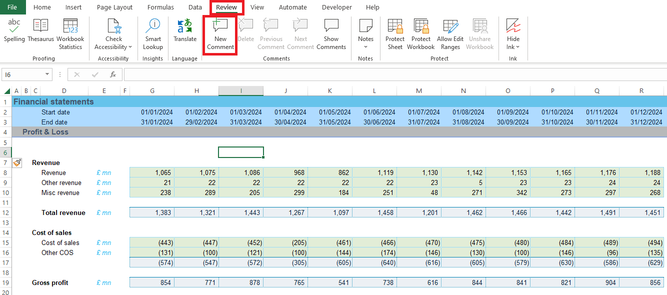
Go to an empty cell (in this example we used I6), on the Review tab of the ribbon click on “New Comment” and enter a comment such as “Inconsistent logic – to review” and press CTRL+ENTER to enter it. (Note we will delete the comment from this cell later.)

Click on Review Tab, then New Comment:

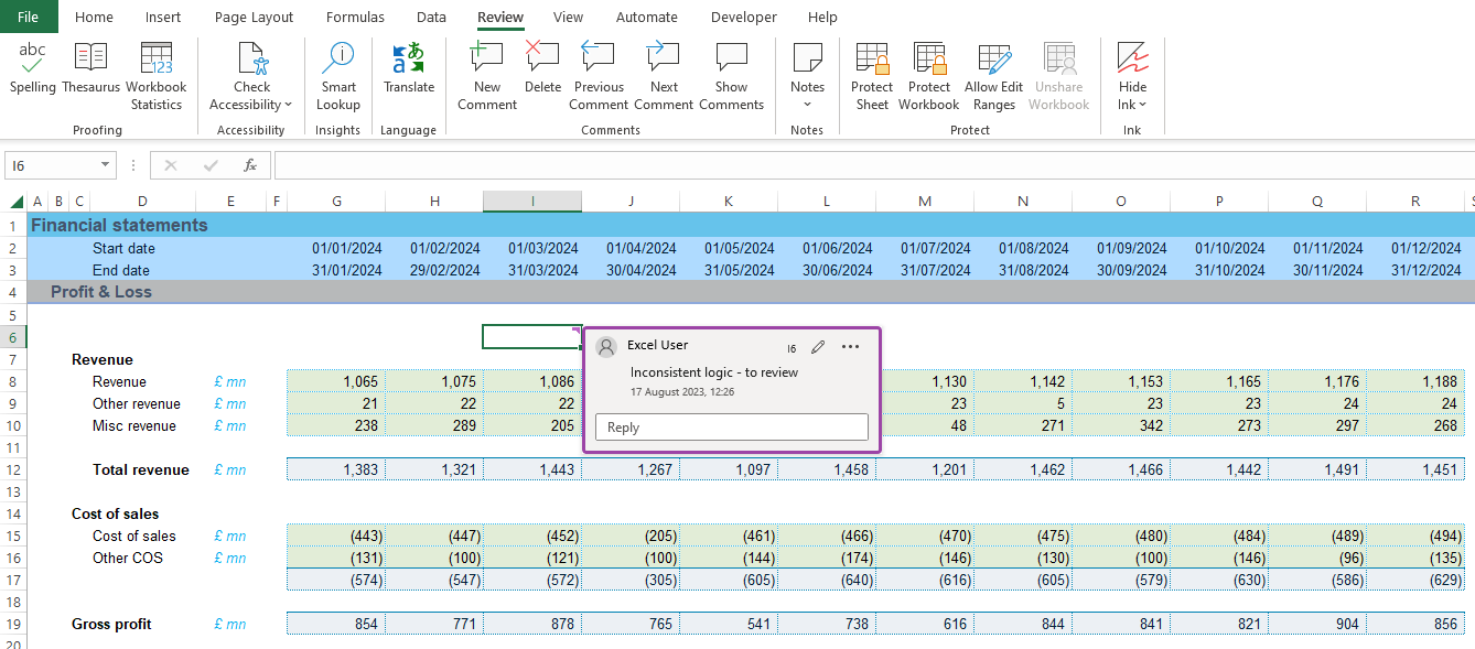
Enter a generic comment to follow up on

Step 2

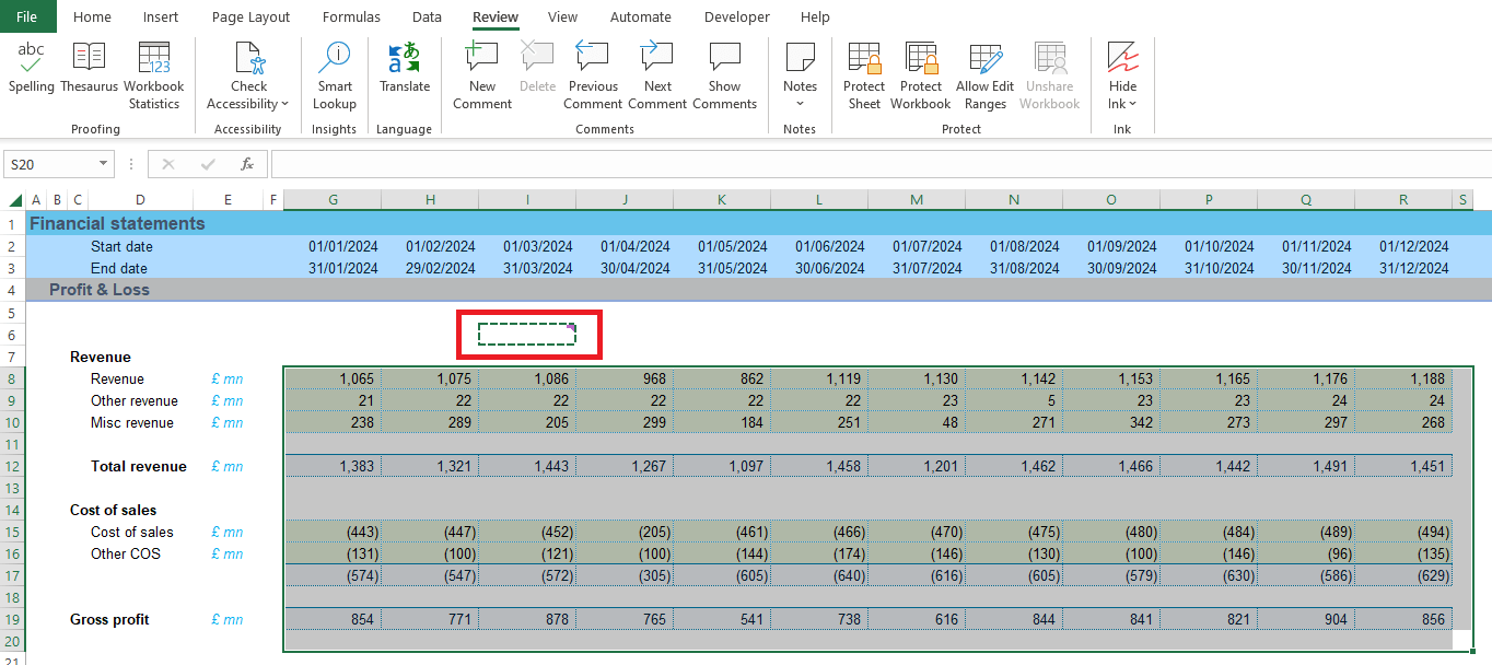
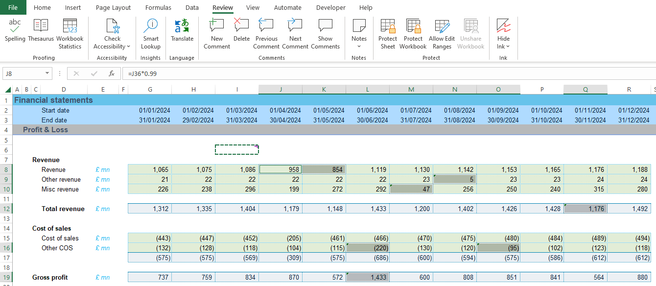
Select that cell and press CTRL+C to copy it and then select all the rows (or columns) in which you want to find inconsistencies.

Copy the cell with the generic comment, and then select the cells to review:

Step 3

Open Go To Special using F5, ALT+S, and then go to either row or column differences and press OK

Use Go To Special to find Row Differences:

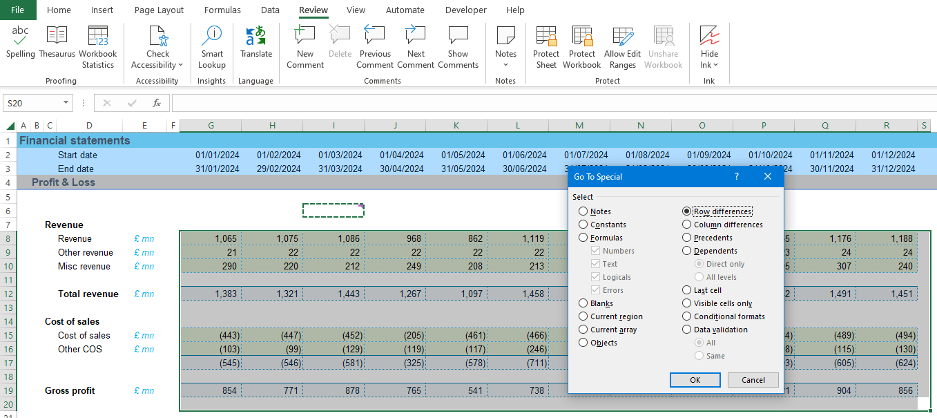
The row differences become selected

Step 4

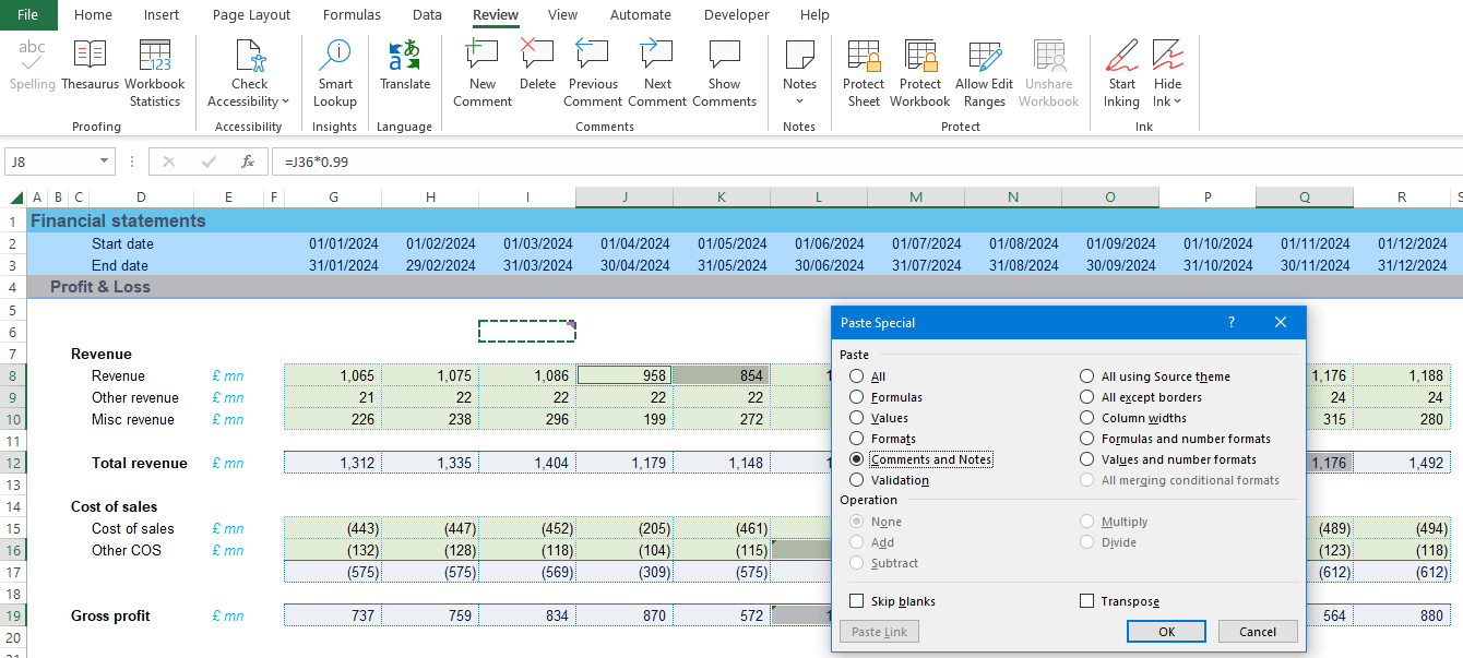
The selection in Excel will now cover all the cells which are inconsistent, and you can now do a “paste special” ALT+E,S" then click on “Comments and Notes”. Now that comment “Inconsistent logic – to review” is marked on all the cells. You can optionally also colour them pink at this point.

Open the paste special menu and select “Comments and Notes”

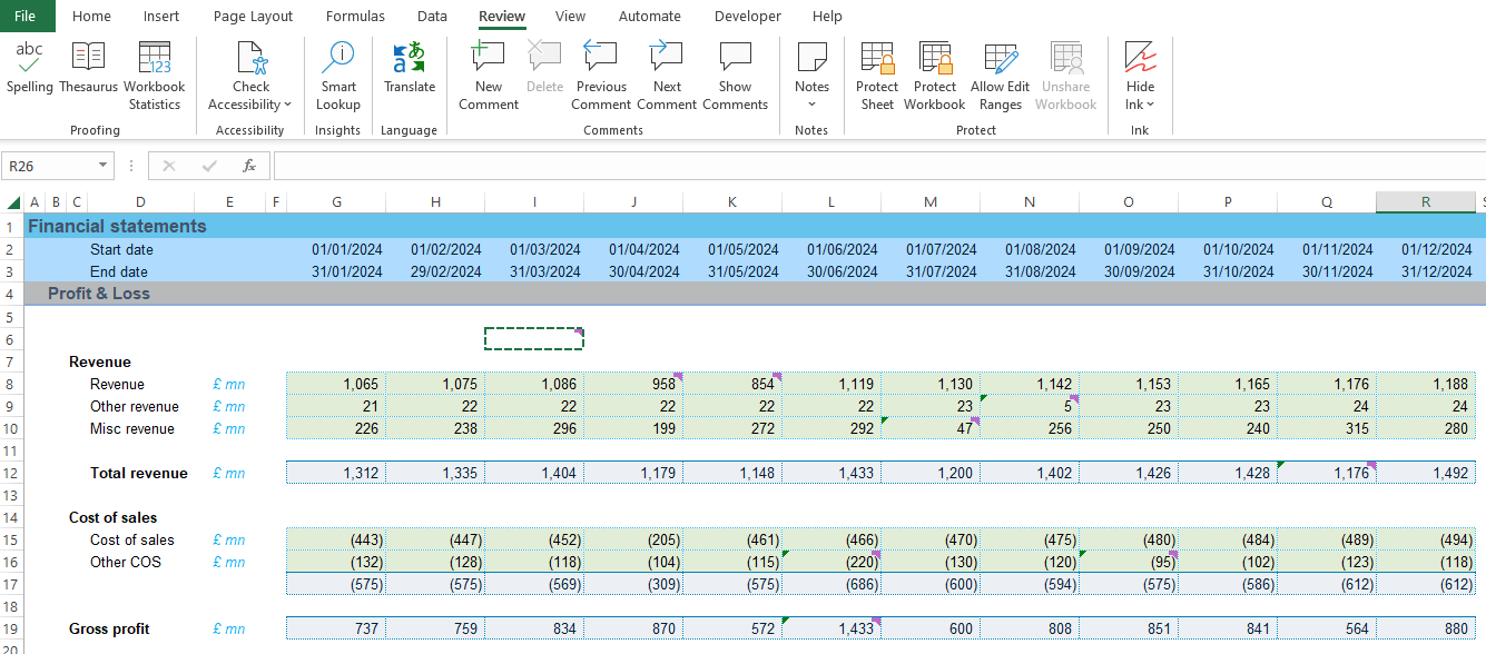
The comments have been applied to all the selected cells – see purple tabs in the top right corners

Step 5

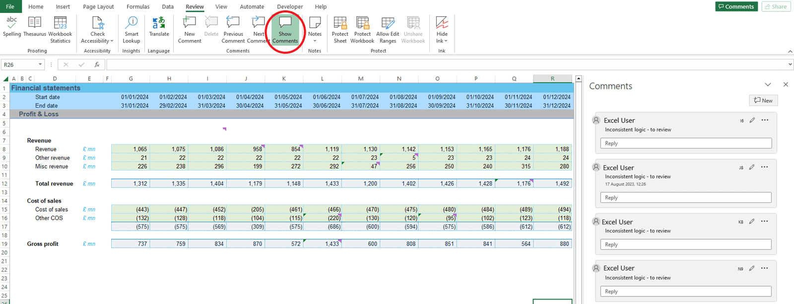
You can now use the “Next Comment” and “Previous Comment” buttons on the Review tab of the ribbon to cycle through each instance of inconsistent logic and address, as necessary. (Don’t forget to delete the temporary generic comment from cell I6)

Use Next / Previous comment buttons, or the Show Comments button to show and navigate through the comments.

Conclusion

Clearly this is not intended to be a substitute for a professional financial model review, but it’s a technique using built in Excel functions which you might find useful. I genuinely hope that this series has proven helpful to some people out there. As always, if you have any comments or questions on this or anything else financial modelling related, please reach out directly or at excel@icaew.com