How can “GO TO SPECIAL” help you understand a spreadsheet?

Sometimes we have to pick up a worksheet which has been prepared by someone else at our firm or maybe elsewhere. Hopefully, they have applied the principles from the ICAEW 20 Principles of Good Spreadsheet Practice, but unfortunately this isn’t always the case. Indeed, sometimes we get a spreadsheet where labels are patchy, the data flow is not clear, there’s no distinguishing formatting and you’ve no idea what's an input, what’s a calculation, where the logic is consistent, and where it changes.

It would really help our understanding of such a sheet if there was a way to colour in the cells according to what is in them. There are specialist software tools available, at a price, which can help with ‘mapping’ a spreadsheet which do exactly that. However, there’s actually quite a lot which can be done using native Excel tools, combined with a little knowledge and the right techniques.

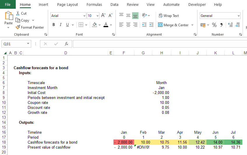
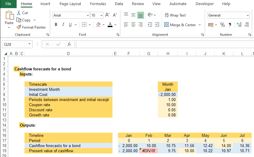
Starting point – Here’s an example of a worksheet which includes no indication on what is formulae, what are constants etc, there is just some conditional formatting applied on row 18:

The concept is use go to special to tool to select different types of cells and colour them according to what is in them to give you a ‘map’ of the worksheet using only native Excel tools. The steps below will get you well on the way.

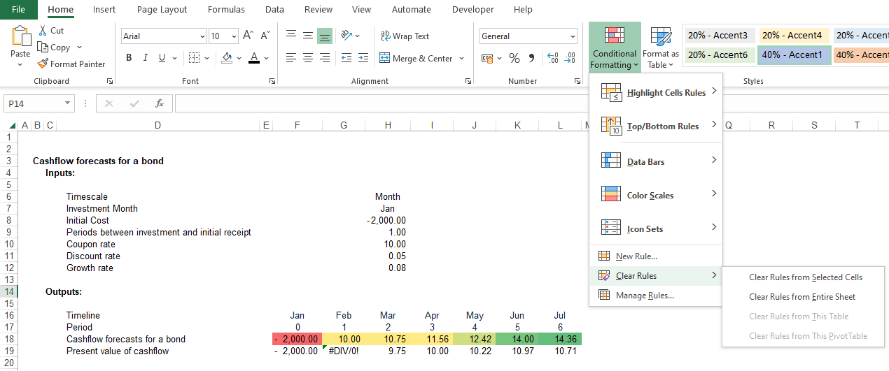
Step 1 – Creating a blank canvas. Some worksheets may already have formatting applied to them, so it’s a good idea to select all the cells, unhide the rows and columns, format the cells using “No Fill” as the background colour, and also delete all conditional formatting rules. (This can be done by clicking on Conditional Formatting on the ribbon, then Clear Rules, …from Entire Worksheet.) This should leave you with a sheet where you can see all the cells and they are not coloured in.

Clearing conditional formatting from the sheet

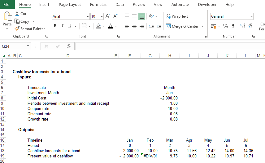
Conditional formatting is gone:

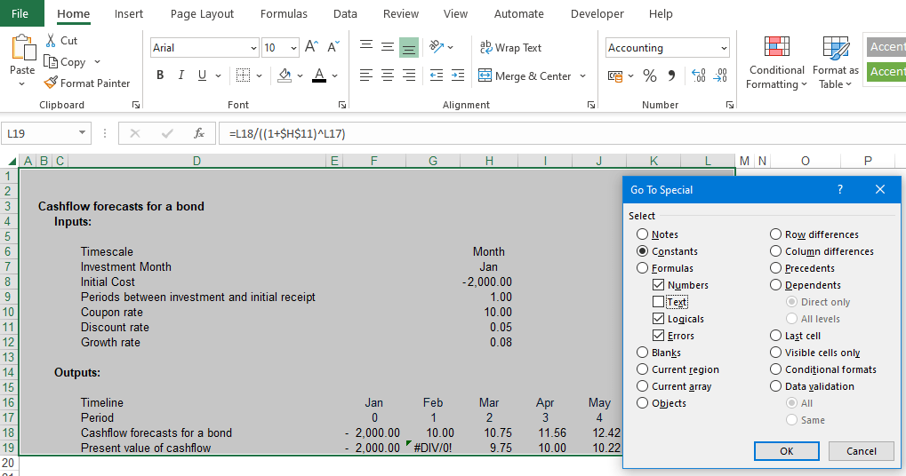
Step 2 – Colour constants. First select all the cells, open the go to special menu (F5, ALT+S) and click on “Constants”, untick “Text”, and leave the other 3 ticked, and click on OK. So long as there were some constants on the sheet they will now be selected. Without clicking on the worksheet (and therefore losing your selection) you can click on the ribbon and on the Home tab go to cell formatting and fill the cells with a light-yellow colour. Now select the whole sheet again, use go to special to select Constants and this time only select “Text”, once again use cell formatting to fill in a slightly darker shade of yellow.

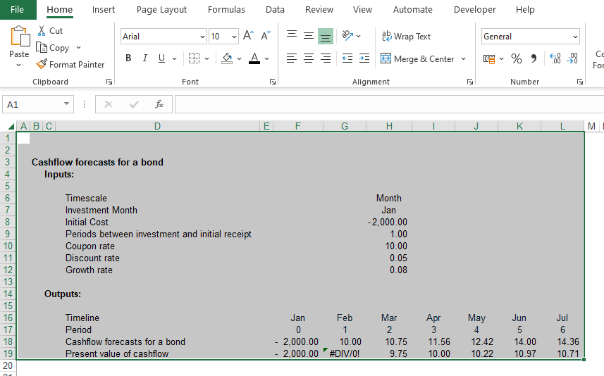
Select entire sheet:

Use Go To Special to select all non-text constants:

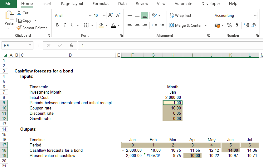
Then format the selected non-text constants in light yellow:

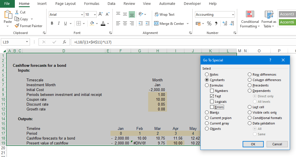
Use Go To Special to select all text constants:

Then format the selected text constants in darker yellow:

Step 3 – Colour formulae. Finally, you can select all the cells, then use go to special to select all the formulae cells and then colour them, say light blue. At this stage you may also want to repeat this step but instead of selecting all formulae types, only select errors and colour them in a share of light red.

Select entire sheet and use Go To Special to select all formulas:

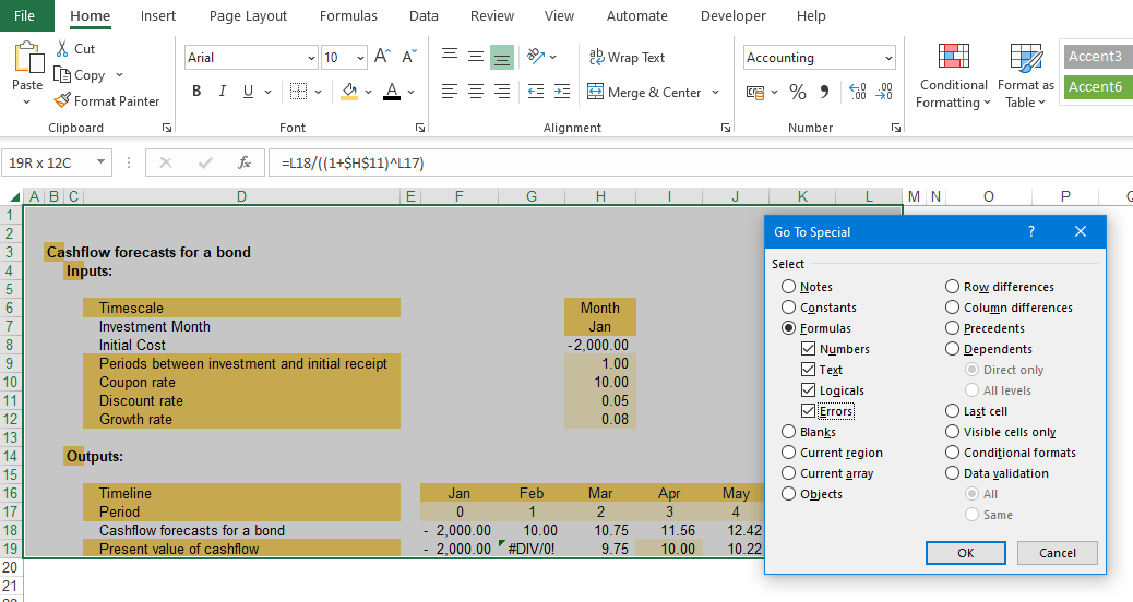
Then format the selected formulas in light blue:

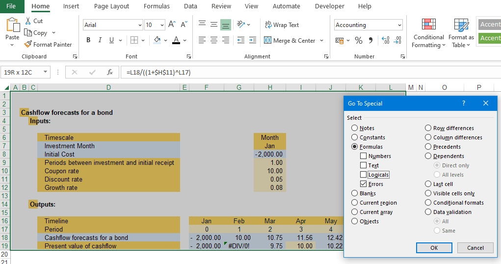
Select entire sheet and use Go To Special to select formulas which evaluate to error values:

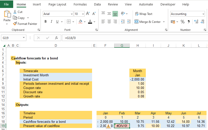
Then format the formulas which evaluate to an error in red:

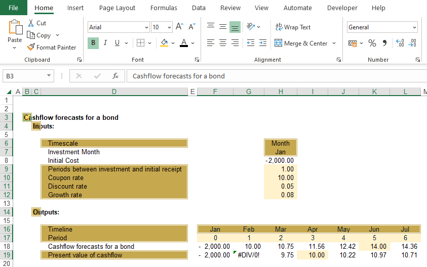
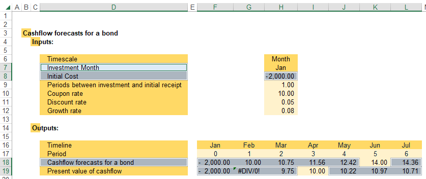
The worksheet is now much more transparent because you can clearly see where the text inputs, the numerical inputs, formulae cells, and errors are.

Result – The final result is a much clearer indication what each cell actually is. In this case it has shown that some of the labels are actually formulas (cells D7:D8) and that some of the cells which looked like formulas are actually hard coded constant inputs (cells K18 and H19).

This is a really good start to understanding a worksheet, but there are opportunities to go a bit further – for example using a similar technique to find and colour all external links. (A detailed explanation is outside the scope of this article but in brief you can do this by using find tool CTRL+F, then look within formulae on the sheet for ‘!’, click on Find All then in the results window use CTRL+A to select all the cells in which ‘!’ was found and then re-colour those.) I’m sure you will also think of other ways you can colour up the worksheet, if you have any gems, please drop me a line!

The final part of this three-article series will look at how to use the row and column differences function to identify and highlight cells where formulae change and then how to mark them for review. Until then, I hope this has been helpful. If you have any comments or questions on this or anything else financial modelling related, please reach out directly or at excel@icaew.com.