Comparing SUMIF, SUMIFS and SUMPRODUCT

Sometimes we wish to aggregate (ie, usually sum) certain values if they meet a particular condition (criterion), or in more complex situations, multiple conditions (criteria). With the demise of the conditional sum wizard in Excel 2010 and anyone under the age of 150 no longer recalling the DBASE functions, assuming you want a generic formulaic solution, the three most common solutions involve:

1. SUMIF
2. SUMIFS
3. SUMPRODUCT

I have ruled out Power Query and dynamic array calculations here. These above variations will work and refresh automatically in all versions of Excel supported presently.

Let’s look at these three functions in turn to see which you should use when – with examples to demonstrate how and why.

Let’s assume I want to summarise the sales made by my business that meet a single condition (eg, sales for a particular business unit). SUMIF happily works here.

The SUMIF function is designed precisely for this situation. It sums values based upon a single criterion. This makes it particularly useful for situations where you need to filter data according to one specific condition and calculate the corresponding sum.

Its syntax is as follows:

SUMIF(range, criterion, [sum_range])

where:

• range: this is the range of cells that Excel will evaluate based upon the condition specified. This range contains the values to be filtered
• criterion: the condition or test applied to the range. It can be a number, expression, text or cell reference. For example, “Product A", ">100” or even “<=”&G5
• sum_range (optional): this the range of cells to sum. If omitted, Excel sums the values in the range that meets the criterion.

There are pros and cons to using this age-old function. Advantages include:

• SUMIF is simple and efficient for single-condition scenarios
• it is easy to learn and implement due to its straightforward syntax
• it is useful for quick data analysis when only one criterion needs to be considered.

There are “areas for opportunity” too:

• SUMIF is limited to handling one condition, making it unsuitable for more complex analysis, although this can be “bulldozed” (see below)
• it does not support logical operators for combining multiple criteria directly.

It should also be noted that if range and an explicitly defined sum_range do not have precisely the same dimensions, sum_range is deemed to have the same dimensions as range, with the range starting with the two ranges sharing the same top left-hand corner cell. The price you pay is the formula becomes volatile, which means it will recalculate whenever anything changes in Excel, which can lead to memory issues. I can’t remember why though (groan – Ed.).

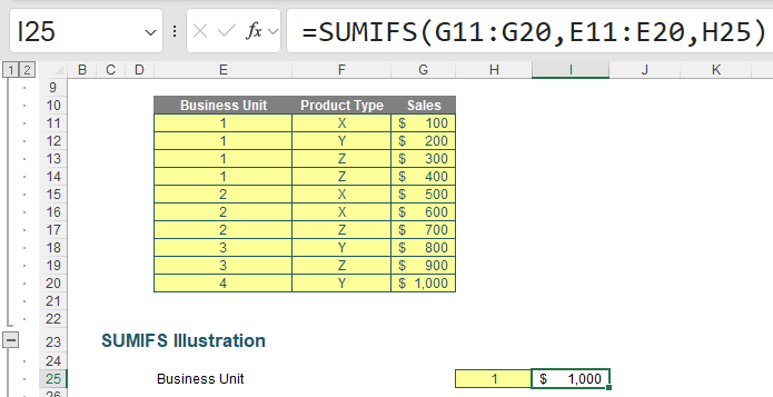
Let’s consider the following example:

To find the sales for Business Unit 1 in the above example, we would type

=SUMIF(E11:E20, H25, G11:G20)

(which is $1,000). But what if you wanted to find the total sales of Product Z in Business Unit 1 using a formula as in the following example?

That’s two criteria and SUMIF will not work with multiple conditions. There are other alternatives. One approach is to add a helper column, “Mega-Criterion” which concatenates columns E and F using the formula

=E11&F11

in cell G11, for instance. It is then trivial to use SUMIF, viz.

=SUMIF(G11:G20, H25&H26, H11:H20)

It is a little 'clunky' (that’s a technical term, do look it up). Is there a better way?

Fortunately, there is. Since Excel 2007, SUMIFS expands on SUMIF by allowing multiple conditions (criteria) to be applied simultaneously. It is ideal for scenarios that require filtering and then aggregating data based upon two or more criteria. Its syntax is:

SUMIFS(sum_range, criteria_range1, criteria1, [criteria_range2, criteria2,] ...)

where:

• sum_range: the range of cells to sum based upon the criteria
• criteria_range: the range of cells to evaluate for each condition. Multiple criteria ranges may be specified
• criteria: the conditions applied to each criteria range. Each condition can be a number, text, expression or cell reference.

The advantages for SUMIFS include:

• the function handles complex scenarios involving multiple conditions
• It provides flexibility for combining logical criteria, enabling more refined data analysis
• SUMIFS ensures accuracy when filtering data based upon multiple factors.

Disadvantages include:

• SUMIFS can become unwieldy and difficult to manage with numerous conditions and large datasets
• it requires all ranges to have the same size, which can lead to errors if not carefully structured (this differs from how SUMIFS works).

SUMIFS provides a simple mechanism for our multiple conditions example:

=SUMIFS(G11:G20, E11:E20, G25, F11:F20, G26)

No concatenation is required in this instance and this works fine if the criteria ranges are all of similar dimensions (eg, if one range is 1 column x 8 rows, then all ranges must be 1 row x 8 columns).

This begs the question, do we still need SUMIF? Personally, I think the answer is no. There is no need to change pre-existing formulae, but if we had a new calculation, I would recommend using SUMIFS rather than SUMIF. For example, let’s return to our original illustration:

=SUMIFS(G11:G20, E11:E20, H25)

The order may not be what we would normally expect, but if we need to add more conditional later, we simply add more arguments to the end of the formula. SUMIF becomes redundant.

There is another benefit of SUMIFS. This solution ignores the text whether it forms part of the answer or not. Since SUMIFS will use the conditions to isolate only matching values that should be summed, it also has the benefit of ignoring items like #N/A in unused data that may cause errors.

Do note that if the #N/A result occurs in the data, there are other ways to get around this issue. Did you know that you can incorporate error results into your conditions? You could try the following for example:

=SUMIFS(G11:G20, E11:E20, H25, F11:F20, "< />#N/A")

The last argument ensures that the #N/A results will be ignored, regardless of whether they form part of your target data. You could repeat this with any other error results as well, though this may result in a very long formula if you don’t consider shortcuts. 

It may be going out of favour with the advent of dynamic arrays but note every version of Excel carries this calculation engine presently. For those who do not know it, SUMPRODUCT(array1 * array2 * ...) appears quite humble upon first glance.

SUMPRODUCT calculates the sum of the products of corresponding values in arrays or ranges. It can also be used for conditional summation when combined with logical expressions. Its syntax is:

SUMPRODUCT(array1, [array2,] ...)

where:

• array: represent the range(s) or array(s) for aggregation
• logical expressions can be included to create complex conditions
• different delimiters (not just commas) may be employed in the SUMPRODUCT syntax.

Advantages in this instance include:

• this function is surprisingly versatile (so much a favourite of mine I named my company after it!), allowing calculations across multiple arrays or ranges
• it supports advanced conditional logic using Boolean operations
• it eliminates the need for array formulae in many instances
• it is capable of handling weighted averages, dynamic calculations, different array dimensions, and plenty more.

Perceived disadvantages include:

• it requires careful handling of arrays and logical expressions to avoid errors
• data types need to be considered carefully: values that look like numbers but are text can cause incorrect answers and / or errors
• it can be computationally intensive for large datasets or complex scenarios and has been demonstrated to use much more resource than equivalent SUMIF or SUMIFS formulae
• it struggles more with errors in the ranges than its SUMIFS counterpart. There is no “one technique" fits all solution to deal with errors in dependent ranges (unlike SUMIFS) and it is recommended your data is cleaned first before applying SUMPRODUCT.

Let’s go back to basics first. Consider the following sales report:

The sales in column G are simply the product of columns E and F, eg, the formula in cell G11 is simply =E11*F11. Then, to calculate the entire amount cell G18 sums column G. This could all be performed much quicker using the following formula:

=SUMPRODUCT(E11:E16, F11:F16)

or

=SUMPRODUCT(E11:E16 * F11:F16)

ie, SUMPRODUCT does exactly what it says on the tin: it sums the individual products.

How does this help the cause? It is all to do with the properties of TRUE and FALSE in Excel, namely:

• TRUE*number = number (e.g. TRUE*7 = 7)
• FALSE*number = 0 (e.g. FALSE*7=0).

In our earlier example (repeated below):

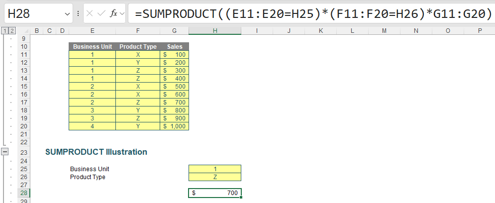
=SUMPRODUCT((E11:E20=H25) * (F11:F20=H26) * G11:G20)

this formula returns the Sales where the Business Unit is 1 and the Product Type is Z. Note that

=SUMPRODUCT((E11:E20=H25), (F11:F20=H26), G11:G20)

gives the wrong answer ($0). This is because the Boolean logic needs to be multiplied. Using the comma delimiter will give the wrong answer as text ranges will be deemed to have zero value.

Notice that SUMPRODUCT is not an array formula although it is an array function. Therefore, as explained above, it can use a lot of memory making the calculation speed of the file slow down.

Used sparingly, however, it can be a highly versatile addition to the modeller’s repertoire. It is a sophisticated function, but once you understand how it works, you can start to use SUMPRODUCT for a whole array of problems (pun intended!).

For example, with SUMPRODUCT, you can manipulate criteria in ways that simply aren’t straightforward with SUMIF or SUMIFS, eg,

=MONTH(D11:D20) = 12

You can also undertake array multiplication with arrays of different sizes, eg,

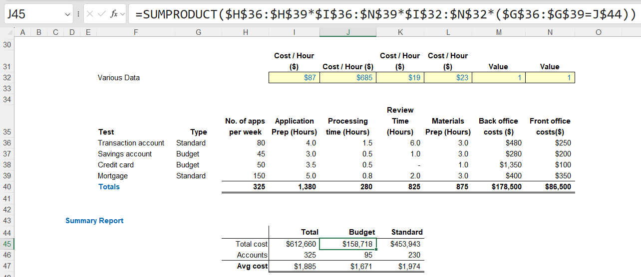
=SUMPRODUCT($H$36:$H$39 * $I$36:$N$39 * $I$32:$N$32 * ($G$36:$G$39 = J$44))

This formula (in black) will aggregate the total costs by taking the number of appointments multiplied by the hours required per appointment multiplied by the hourly rate. Note that the number of rows in the hours required array ($I$36:$N$39) equals the number of rows in the number of appointments per week vector ($H$36:$H$39). Also, note that the number of columns in the hours required array ($I$36:$N$39) equals the number of columns in the input vector ($I$32:$N$32). This must hold for the formula to work.

The condition in red determines whether “Budget” or “Standard” account types should be considered – hence all the anchoring. Again, note that the number of rows in the hours required array ($I$36:$N$39) equals the number of rows in the type of account vector condition ($G$36:$G$39 = J$44).

It is complex, but powerful – and that pretty much sums up SUMPRODUCT.

SUMIF, SUMIFS and SUMPRODUCT each serve distinct purposes within Excel. SUMIF is straightforward and efficient for single conditions but perhaps should now be consigned as a legacy function. SUMIFS is probably the simplest (best?) all-rounder for handling multiple criteria as long as the dimensions of each condition are consistent. SUMPRODUCT provides unmatched versatility for advanced calculations, but formulae can be more opaque and slower.

Only by understanding their unique strengths and limitations can you fully leverage these functions for your day-to-day modelling needs. Do master them.